This demo studies a sizing optimisation problem for an inverse truss bridge and shows how the dolfiny interface to PETSc/TAO can be used to minimise compliance under a volume constraint. It demonstrates a linear elastic truss model written in UFL, the generation of braced truss meshes, and the optimisation workflow for the bar cross-sectional areas.
In particular, this demo emphasizes:
truss meshes as an instance of (interval cells embedded in ),
vertex integrals (
dPmeasure) for concentrated point loads in variational form,sizing optimisation with TAO’s MMA and CONLIN algorithms via
dolfiny.taoproblem,volume-equality constraint expressed in reduced form.
Source
import argparse
import warnings

from mpi4py import MPI
from petsc4py import PETSc

import dolfinx
import dolfinx.fem.petsc
import ufl

import matplotlib.pyplot as plt
import matplotlib_inline
import numpy as np
import pyvista as pv

import dolfiny
import dolfiny.taoproblem
from dolfiny.expression import normalize

warnings.filterwarnings("error")

parser = argparse.ArgumentParser(description="Truss sizing demo")
parser.add_argument(
    "-a",
    "--algorithm",
    choices=["conlin", "mma"],
    default="mma",
    help="Choose optimisation algorithm",
)
args, _unknown = parser.parse_known_args()
Generation of truss meshes
Truss structures make up an interesting example of the concept of geometric- and
topological dimension, let those be denoted as and , which is also used throughout
DOLFINx Baratta et al., 2023.
The geometric dimension is the dimension of the space in which the mesh is embedded, and , and the topological dimension is the dimension of the cells of the mesh in the reference configuration, for the reference cell of .
The usual finite element text-book setting applies to the case , for example a triangle mesh is only considered in and not in .
Trusses are made up of lines, or, domain inspecifc, intervals, which are one-dimensional entities and form planar or volumetric structures, . Here, we consider the volumetric case, .
The bridge dimensions (length, height, width) are all in meters and we create
the truss mesh from the edges of a (regular) hexahedral mesh, with trusses of size , and
introduce all possible bracings to it.
This is what the create_truss_x_braced_mesh functionality simplifies.
Given a hexehedral mesh, it generates the edge skeleton together with all possible bracings.
Source
comm = MPI.COMM_WORLD

dim = np.array([100, 20, 10], dtype=np.float64)
elem_size = 5
mesh = dolfiny.mesh_generation.create_truss_x_braced_mesh(
    dolfinx.mesh.create_box(
        MPI.COMM_SELF,
        [np.zeros_like(dim), dim],
        (dim / elem_size).astype(np.int32),  # type: ignore
        dolfinx.mesh.CellType.hexahedron,
    )
    if comm.rank == 0
    else None
)
We create one functionspace for the displacement field and one for the cross sectional area of the trusses, which we model as constant over each element, so .
Source
V_u = dolfinx.fem.functionspace(mesh, ("P", 1, (3,)))
u = dolfinx.fem.Function(V_u, name="displacement")

V_s = dolfinx.fem.functionspace(mesh, ("DG", 0))
s = dolfinx.fem.Function(V_s, name="cross-sectional-area")
Boundary conditions and load surface
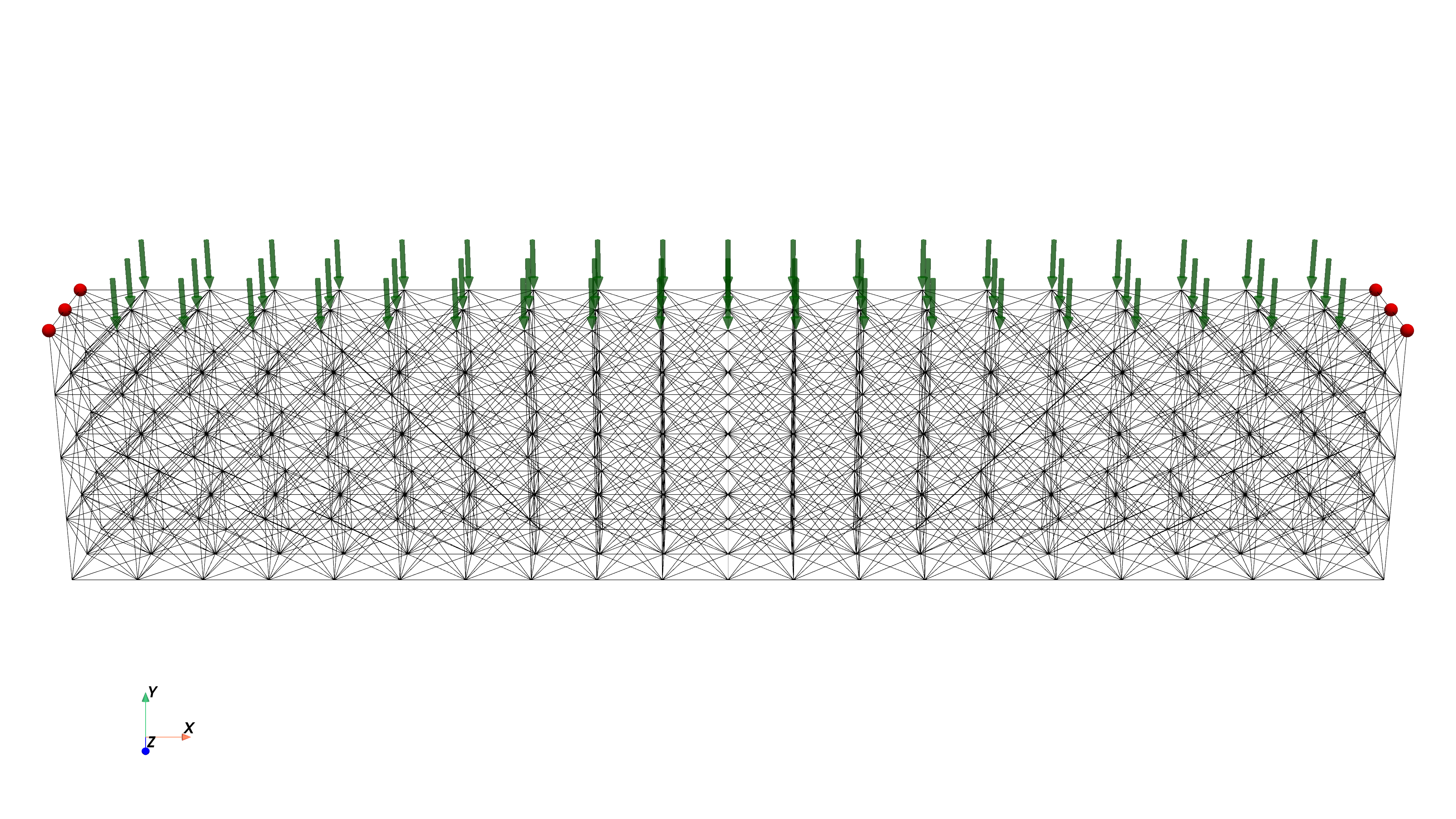
For the realisation of an inverse truss bridge, we will fix the trusses on the left and right top edges and apply a vertical load, i.e. in -direction, on the bridge deck, which we assume to span the whole upper surface/side of the truss mesh, excluding the fixed edges.
Source
mesh.topology.create_connectivity(0, 1)
vertices_fixed = dolfinx.mesh.locate_entities(
    mesh,
    0,
    lambda x: (np.isclose(x[0], 0) | np.isclose(x[0], dim[0])) & np.isclose(x[1], dim[1]),
)

dofs_fixed = dolfinx.fem.locate_dofs_topological(V_u, 0, vertices_fixed)
bcs = [dolfinx.fem.dirichletbc(np.zeros(3, dtype=np.float64), dofs_fixed, V_u)]

vertices_load = dolfinx.mesh.locate_entities(
    mesh, 0, lambda x: np.isclose(x[1], dim[1]) & np.greater(x[0], 0) & np.less(x[0], dim[0])
)
meshtags = dolfinx.mesh.meshtags(mesh, 0, vertices_load, 1)
vertices_load_local = vertices_load[vertices_load < mesh.topology.index_map(0).size_local]

pv.set_jupyter_backend("static")
pv_grid = pv.UnstructuredGrid(*dolfinx.plot.vtk_mesh(mesh))
plotter = pv.Plotter(window_size=[3840, 2160])
plotter.add_mesh(pv_grid, color="black", line_width=1.5)

for v in vertices_load:
    v_coords = mesh.geometry.x[v]
    arrow = pv.Arrow(start=v_coords + np.array([0, 4, 0]), direction=[0, -1, 0], scale=4)
    plotter.add_mesh(arrow, color="green", opacity=0.5)

for v in vertices_fixed:
    v_coords = mesh.geometry.x[v]
    sphere = pv.Sphere(radius=0.5, center=v_coords)
    plotter.add_mesh(sphere, color="red")

plotter.view_xy()
plotter.add_axes()
plotter.camera.elevation += 20
plotter.camera.zoom(1.7)
plotter.show()
plotter.close()
plotter.deep_clean()
Figure 1:Truss mesh with fixed supports (red spheres) and load-application vertices (green arrows).
Truss model and forward problem
We rely on a linear elastic truss model, following Bleyer, 2024. We choose a Young’s modulus of and apply a total load of , equally distributed across the loaded nodes.
Source
tangent = normalize(ufl.Jacobian(mesh)[:, 0])

E = 200.0 * 1e9  # [E] = Pa = N/m^2
ε = ufl.dot(ufl.dot(ufl.grad(u), tangent), tangent)  # strain
N = E * s * ε  # normal_force

dP = ufl.Measure("dP", domain=mesh, subdomain_data=meshtags)
total_load = 300 * 1e3
num_load_vertices = comm.allreduce(vertices_load_local.size)
F = ufl.as_vector([0, -total_load / num_load_vertices, 0])
compliance = ufl.inner(F, u) * dP(1)

E = 1 / 2 * ufl.inner(N, ε) * ufl.dx - compliance

a = ufl.derivative(ufl.derivative(E, u), u)
L = ufl.derivative(compliance, u)

state_solver = dolfinx.fem.petsc.LinearProblem(
    a,
    L,
    bcs=bcs,
    u=u,
    petsc_options={
        "ksp_type": "preonly",
        "pc_type": "lu",
        "pc_factor_mat_solver_type": "mumps",
        "ksp_error_if_not_converged": "True",
        "mat_mumps_cntl_1": 0.0,  # Disable relative pivoting threshold
    },
    petsc_options_prefix="state_solver",
)
Output
Optimisation of cross-sectional areas
The truss sizing optimisation problem from Christensen & Klarbring, 2009 that we study is given (in reduced form) by
where is the unique displacement field associated with a given sizing .
For the bounds of the truss cross sectional area we consider an upper bound of and set the the lower bound to .
Source
compliance_form = dolfinx.fem.form(compliance)


@dolfiny.taoproblem.sync_functions([s])
def C(tao, x) -> float:
    state_solver.solve()
    return comm.allreduce(dolfinx.fem.assemble_scalar(compliance_form))  # type: ignore


# p = -u
p = dolfinx.fem.Function(V_u)
gx = dolfinx.fem.form(ufl.derivative(ufl.derivative(E, u, p), s))


@dolfiny.taoproblem.sync_functions([s])
def JC(tao, x, J):
    state_solver.solve()

    J.zeroEntries()
    p.x.array[:] = -u.x.array

    dolfinx.fem.petsc.assemble_vector(J, gx)
    J.ghostUpdate(addv=PETSc.InsertMode.ADD, mode=PETSc.ScatterMode.REVERSE)


s_max = np.float64(1e-2)
s_min = np.float64(1e-3 * s_max)
max_vol = comm.allreduce(
    dolfinx.fem.assemble_scalar(dolfinx.fem.form(dolfinx.fem.Constant(mesh, s_max) * ufl.dx))
)
volume_fraction = 1 / 20
h = [s / max_vol / volume_fraction * ufl.dx <= 1]
s.x.array[:] = 1 / 100 * s_max

opts = PETSc.Options("truss")  # type: ignore
opts["tao_type"] = "python"
opts["tao_monitor"] = ""
opts["tao_max_it"] = (max_it := 50)
if args.algorithm == "conlin":
    opts["tao_python_type"] = "dolfiny.conlin.CONLIN"
else:  # mma
    opts["tao_python_type"] = "dolfiny.mma.MMA"
    opts["tao_mma_move_limit"] = 0.05
    opts["tao_mma_subsolver_tao_max_it"] = 30

problem = dolfiny.taoproblem.TAOProblem(
    C, [s], bcs=bcs, J=(JC, s.x.petsc_vec.copy()), h=h, lb=s_min, ub=s_max, prefix="truss"
)


def monitor(tao, comp, volume):
    it = tao.getIterationNumber()
    comp[it] = tao.getObjectiveValue()
    volume[it] = dolfinx.fem.assemble_scalar(dolfinx.fem.form(h[0].lhs))


comp = np.zeros(max_it, np.float64)
volume = np.zeros(max_it, np.float64)

if comm.size == 1:
    problem.tao.setMonitor(monitor, (comp, volume))
problem.solve()

state_solver.solve()
Output
# TAO 0 (ITERATING)
# sub 0 [ 2k] |x|=5.117e-03 |J|=1.025e+07 (cross-sectional-area)
# all |x|=5.117e-03 |J|=1.025e+07 |h|=0.000e+00 |Jh|=0.000e+00 f=1.961e+04
# TAO 1 (ITERATING)
# sub 0 [ 2k] |x|=2.680e-02 |J|=2.897e+05 (cross-sectional-area)
# all |x|=2.680e-02 |J|=2.897e+05 |h|=8.000e-01 |Jh|=3.984e+01 f=3.316e+03
# TAO 2 (ITERATING)
# sub 0 [ 2k] |x|=3.489e-02 |J|=1.214e+05 (cross-sectional-area)
# all |x|=3.489e-02 |J|=1.214e+05 |h|=8.368e-02 |Jh|=3.984e+01 f=2.142e+03
# TAO 3 (ITERATING)
# sub 0 [ 2k] |x|=3.923e-02 |J|=7.770e+04 (cross-sectional-area)
# all |x|=3.923e-02 |J|=7.770e+04 |h|=6.729e-02 |Jh|=3.984e+01 f=1.649e+03
# TAO 4 (ITERATING)
# sub 0 [ 2k] |x|=4.556e-02 |J|=8.016e+04 (cross-sectional-area)
# all |x|=4.556e-02 |J|=8.016e+04 |h|=5.449e-02 |Jh|=3.984e+01 f=1.390e+03
# TAO 5 (ITERATING)
# sub 0 [ 2k] |x|=4.995e-02 |J|=4.299e+04 (cross-sectional-area)
# all |x|=4.995e-02 |J|=4.299e+04 |h|=4.857e-02 |Jh|=3.984e+01 f=1.224e+03
# TAO 6 (ITERATING)
# sub 0 [ 2k] |x|=5.493e-02 |J|=5.084e+04 (cross-sectional-area)
# all |x|=5.493e-02 |J|=5.084e+04 |h|=4.832e-02 |Jh|=3.984e+01 f=1.109e+03
# TAO 7 (ITERATING)
# sub 0 [ 2k] |x|=5.791e-02 |J|=2.629e+04 (cross-sectional-area)
# all |x|=5.791e-02 |J|=2.629e+04 |h|=3.917e-02 |Jh|=3.984e+01 f=1.025e+03
# TAO 8 (ITERATING)
# sub 0 [ 2k] |x|=6.400e-02 |J|=2.687e+04 (cross-sectional-area)
# all |x|=6.400e-02 |J|=2.687e+04 |h|=3.706e-02 |Jh|=3.984e+01 f=9.325e+02
  Iteration information for truss solve.
  0 TAO,  Function value: 19614.4,  Residual: 0.
  1 TAO,  Function value: 3315.56,  Residual: 289728.
  2 TAO,  Function value: 2142.44,  Residual: 121362.
  3 TAO,  Function value: 1648.92,  Residual: 77696.9
  4 TAO,  Function value: 1390.03,  Residual: 80160.9
  5 TAO,  Function value: 1223.78,  Residual: 42986.3
  6 TAO,  Function value: 1109.08,  Residual: 50835.4
  7 TAO,  Function value: 1025.34,  Residual: 26288.2
  8 TAO,  Function value: 932.513,  Residual: 26873.7
# TAO 9 (ITERATING)
# sub 0 [ 2k] |x|=6.679e-02 |J|=1.909e+04 (cross-sectional-area)
# all |x|=6.679e-02 |J|=1.909e+04 |h|=2.624e-02 |Jh|=3.984e+01 f=8.846e+02
# TAO 10 (ITERATING)
# sub 0 [ 2k] |x|=7.119e-02 |J|=1.721e+04 (cross-sectional-area)
# all |x|=7.119e-02 |J|=1.721e+04 |h|=1.803e-02 |Jh|=3.984e+01 f=8.319e+02
# TAO 11 (ITERATING)
# sub 0 [ 2k] |x|=7.406e-02 |J|=1.834e+04 (cross-sectional-area)
# all |x|=7.406e-02 |J|=1.834e+04 |h|=1.140e-02 |Jh|=3.984e+01 f=8.017e+02
# TAO 12 (ITERATING)
# sub 0 [ 2k] |x|=7.550e-02 |J|=1.698e+04 (cross-sectional-area)
# all |x|=7.550e-02 |J|=1.698e+04 |h|=6.276e-03 |Jh|=3.984e+01 f=7.869e+02
# TAO 13 (ITERATING)
# sub 0 [ 2k] |x|=7.800e-02 |J|=1.560e+04 (cross-sectional-area)
# all |x|=7.800e-02 |J|=1.560e+04 |h|=7.674e-03 |Jh|=3.984e+01 f=7.638e+02
# TAO 14 (ITERATING)
# sub 0 [ 2k] |x|=8.042e-02 |J|=2.733e+04 (cross-sectional-area)
# all |x|=8.042e-02 |J|=2.733e+04 |h|=7.190e-03 |Jh|=3.984e+01 f=7.488e+02
# TAO 15 (ITERATING)
# sub 0 [ 2k] |x|=7.972e-02 |J|=1.695e+04 (cross-sectional-area)
# all |x|=7.972e-02 |J|=1.695e+04 |h|=5.554e-03 |Jh|=3.984e+01 f=7.519e+02
# TAO 16 (ITERATING)
# sub 0 [ 2k] |x|=8.286e-02 |J|=1.616e+04 (cross-sectional-area)
# all |x|=8.286e-02 |J|=1.616e+04 |h|=1.256e-02 |Jh|=3.984e+01 f=7.267e+02
# TAO 17 (ITERATING)
# sub 0 [ 2k] |x|=8.459e-02 |J|=1.530e+04 (cross-sectional-area)
  9 TAO,  Function value: 884.561,  Residual: 19086.1
 10 TAO,  Function value: 831.9,  Residual: 17213.2
 11 TAO,  Function value: 801.734,  Residual: 18340.9
 12 TAO,  Function value: 786.914,  Residual: 16978.9
 13 TAO,  Function value: 763.783,  Residual: 15603.5
 14 TAO,  Function value: 748.808,  Residual: 27330.8
 15 TAO,  Function value: 751.909,  Residual: 16953.3
 16 TAO,  Function value: 726.702,  Residual: 16158.5
 17 TAO,  Function value: 713.137,  Residual: 15300.6
# all |x|=8.459e-02 |J|=1.530e+04 |h|=9.076e-03 |Jh|=3.984e+01 f=7.131e+02
# TAO 18 (ITERATING)
# sub 0 [ 2k] |x|=8.625e-02 |J|=1.531e+04 (cross-sectional-area)
# all |x|=8.625e-02 |J|=1.531e+04 |h|=6.239e-03 |Jh|=3.984e+01 f=7.024e+02
# TAO 19 (ITERATING)
# sub 0 [ 2k] |x|=8.817e-02 |J|=1.364e+04 (cross-sectional-area)
# all |x|=8.817e-02 |J|=1.364e+04 |h|=6.252e-03 |Jh|=3.984e+01 f=6.900e+02
# TAO 20 (ITERATING)
# sub 0 [ 2k] |x|=9.017e-02 |J|=1.290e+04 (cross-sectional-area)
# all |x|=9.017e-02 |J|=1.290e+04 |h|=5.602e-03 |Jh|=3.984e+01 f=6.792e+02
# TAO 21 (ITERATING)
# sub 0 [ 2k] |x|=9.085e-02 |J|=1.272e+04 (cross-sectional-area)
# all |x|=9.085e-02 |J|=1.272e+04 |h|=4.684e-03 |Jh|=3.984e+01 f=6.756e+02
# TAO 22 (ITERATING)
# sub 0 [ 2k] |x|=9.095e-02 |J|=1.282e+04 (cross-sectional-area)
# all |x|=9.095e-02 |J|=1.282e+04 |h|=3.681e-03 |Jh|=3.984e+01 f=6.752e+02
# TAO 23 (ITERATING)
# sub 0 [ 2k] |x|=9.136e-02 |J|=1.150e+04 (cross-sectional-area)
# all |x|=9.136e-02 |J|=1.150e+04 |h|=3.492e-03 |Jh|=3.984e+01 f=6.735e+02
# TAO 24 (ITERATING)
# sub 0 [ 2k] |x|=9.168e-02 |J|=1.198e+04 (cross-sectional-area)
# all |x|=9.168e-02 |J|=1.198e+04 |h|=3.710e-03 |Jh|=3.984e+01 f=6.717e+02
# TAO 25 (ITERATING)
# sub 0 [ 2k] |x|=9.173e-02 |J|=1.105e+04 (cross-sectional-area)
# all |x|=9.173e-02 |J|=1.105e+04 |h|=2.905e-03 |Jh|=3.984e+01 f=6.723e+02
 18 TAO,  Function value: 702.44,  Residual: 15307.7
 19 TAO,  Function value: 690.009,  Residual: 13636.7
 20 TAO,  Function value: 679.203,  Residual: 12897.3
 21 TAO,  Function value: 675.623,  Residual: 12722.1
 22 TAO,  Function value: 675.236,  Residual: 12819.9
 23 TAO,  Function value: 673.486,  Residual: 11504.3
 24 TAO,  Function value: 671.741,  Residual: 11977.9
 25 TAO,  Function value: 672.325,  Residual: 11052.9
 26 TAO,  Function value: 669.717,  Residual: 11892.2
# TAO 26 (ITERATING)
# sub 0 [ 2k] |x|=9.207e-02 |J|=1.189e+04 (cross-sectional-area)
# all |x|=9.207e-02 |J|=1.189e+04 |h|=2.930e-03 |Jh|=3.984e+01 f=6.697e+02
# TAO 27 (ITERATING)
# sub 0 [ 2k] |x|=9.192e-02 |J|=1.106e+04 (cross-sectional-area)
# all |x|=9.192e-02 |J|=1.106e+04 |h|=2.255e-03 |Jh|=3.984e+01 f=6.714e+02
# TAO 28 (ITERATING)
# sub 0 [ 2k] |x|=9.232e-02 |J|=1.304e+04 (cross-sectional-area)
# all |x|=9.232e-02 |J|=1.304e+04 |h|=2.630e-03 |Jh|=3.984e+01 f=6.690e+02
# TAO 29 (ITERATING)
# sub 0 [ 2k] |x|=9.202e-02 |J|=1.111e+04 (cross-sectional-area)
# all |x|=9.202e-02 |J|=1.111e+04 |h|=2.285e-03 |Jh|=3.984e+01 f=6.717e+02
# TAO 30 (ITERATING)
# sub 0 [ 2k] |x|=9.251e-02 |J|=1.214e+04 (cross-sectional-area)
# all |x|=9.251e-02 |J|=1.214e+04 |h|=3.350e-03 |Jh|=3.984e+01 f=6.684e+02
# TAO 31 (ITERATING)
# sub 0 [ 2k] |x|=9.254e-02 |J|=1.060e+04 (cross-sectional-area)
# all |x|=9.254e-02 |J|=1.060e+04 |h|=2.472e-03 |Jh|=3.984e+01 f=6.680e+02
# TAO 32 (ITERATING)
# sub 0 [ 2k] |x|=9.270e-02 |J|=1.109e+04 (cross-sectional-area)
# all |x|=9.270e-02 |J|=1.109e+04 |h|=1.509e-03 |Jh|=3.984e+01 f=6.671e+02
# TAO 33 (ITERATING)
# sub 0 [ 2k] |x|=9.270e-02 |J|=1.102e+04 (cross-sectional-area)
# all |x|=9.270e-02 |J|=1.102e+04 |h|=9.261e-04 |Jh|=3.984e+01 f=6.671e+02
# TAO 34 (ITERATING)
# sub 0 [ 2k] |x|=9.261e-02 |J|=1.118e+04 (cross-sectional-area)
# all |x|=9.261e-02 |J|=1.118e+04 |h|=5.980e-04 |Jh|=3.984e+01 f=6.683e+02
# TAO 35 (ITERATING)
# sub 0 [ 2k] |x|=9.269e-02 |J|=1.095e+04 (cross-sectional-area)
# all |x|=9.269e-02 |J|=1.095e+04 |h|=1.029e-03 |Jh|=3.984e+01 f=6.676e+02
 27 TAO,  Function value: 671.428,  Residual: 11061.6
 28 TAO,  Function value: 668.967,  Residual: 13043.8
 29 TAO,  Function value: 671.666,  Residual: 11109.6
 30 TAO,  Function value: 668.425,  Residual: 12137.9
 31 TAO,  Function value: 668.046,  Residual: 10600.1
 32 TAO,  Function value: 667.11,  Residual: 11092.2
 33 TAO,  Function value: 667.134,  Residual: 11017.6
 34 TAO,  Function value: 668.263,  Residual: 11184.8
 35 TAO,  Function value: 667.581,  Residual: 10950.2
# TAO 36 (ITERATING)
# sub 0 [ 2k] |x|=9.275e-02 |J|=1.082e+04 (cross-sectional-area)
# all |x|=9.275e-02 |J|=1.082e+04 |h|=9.733e-04 |Jh|=3.984e+01 f=6.672e+02
# TAO 37 (ITERATING)
# sub 0 [ 2k] |x|=9.281e-02 |J|=1.073e+04 (cross-sectional-area)
# all |x|=9.281e-02 |J|=1.073e+04 |h|=7.591e-04 |Jh|=3.984e+01 f=6.668e+02
# TAO 38 (ITERATING)
# sub 0 [ 2k] |x|=9.288e-02 |J|=1.061e+04 (cross-sectional-area)
# all |x|=9.288e-02 |J|=1.061e+04 |h|=6.380e-04 |Jh|=3.984e+01 f=6.664e+02
# TAO 39 (ITERATING)
# sub 0 [ 2k] |x|=9.292e-02 |J|=1.058e+04 (cross-sectional-area)
# all |x|=9.292e-02 |J|=1.058e+04 |h|=4.288e-04 |Jh|=3.984e+01 f=6.663e+02
# TAO 40 (ITERATING)
# sub 0 [ 2k] |x|=9.295e-02 |J|=1.040e+04 (cross-sectional-area)
# all |x|=9.295e-02 |J|=1.040e+04 |h|=3.030e-04 |Jh|=3.984e+01 f=6.661e+02
# TAO 41 (ITERATING)
# sub 0 [ 2k] |x|=9.296e-02 |J|=1.029e+04 (cross-sectional-area)
# all |x|=9.296e-02 |J|=1.029e+04 |h|=2.525e-04 |Jh|=3.984e+01 f=6.660e+02
# TAO 42 (ITERATING)
# sub 0 [ 2k] |x|=9.298e-02 |J|=1.023e+04 (cross-sectional-area)
# all |x|=9.298e-02 |J|=1.023e+04 |h|=1.225e-04 |Jh|=3.984e+01 f=6.659e+02
# TAO 43 (ITERATING)
# sub 0 [ 2k] |x|=9.301e-02 |J|=1.027e+04 (cross-sectional-area)
# all |x|=9.301e-02 |J|=1.027e+04 |h|=7.149e-05 |Jh|=3.984e+01 f=6.659e+02
# TAO 44 (ITERATING)
# sub 0 [ 2k] |x|=9.296e-02 |J|=1.020e+04 (cross-sectional-area)
# all |x|=9.296e-02 |J|=1.020e+04 |h|=6.749e-05 |Jh|=3.984e+01 f=6.660e+02
 36 TAO,  Function value: 667.153,  Residual: 10822.1
 37 TAO,  Function value: 666.849,  Residual: 10733.5
 38 TAO,  Function value: 666.431,  Residual: 10607.4
 39 TAO,  Function value: 666.256,  Residual: 10584.2
 40 TAO,  Function value: 666.078,  Residual: 10398.2
 41 TAO,  Function value: 665.969,  Residual: 10287.8
 42 TAO,  Function value: 665.898,  Residual: 10230.6
 43 TAO,  Function value: 665.936,  Residual: 10273.4
 44 TAO,  Function value: 666.018,  Residual: 10201.1
# TAO 45 (ITERATING)
# sub 0 [ 2k] |x|=9.302e-02 |J|=1.025e+04 (cross-sectional-area)
# all |x|=9.302e-02 |J|=1.025e+04 |h|=2.009e-04 |Jh|=3.984e+01 f=6.659e+02
# TAO 46 (ITERATING)
# sub 0 [ 2k] |x|=9.302e-02 |J|=1.023e+04 (cross-sectional-area)
# all |x|=9.302e-02 |J|=1.023e+04 |h|=1.783e-04 |Jh|=3.984e+01 f=6.659e+02
# TAO 47 (ITERATING)
# sub 0 [ 2k] |x|=9.304e-02 |J|=1.035e+04 (cross-sectional-area)
# all |x|=9.304e-02 |J|=1.035e+04 |h|=9.636e-05 |Jh|=3.984e+01 f=6.659e+02
# TAO 48 (ITERATING)
# sub 0 [ 2k] |x|=9.306e-02 |J|=1.032e+04 (cross-sectional-area)
# all |x|=9.306e-02 |J|=1.032e+04 |h|=9.086e-05 |Jh|=3.984e+01 f=6.660e+02
# TAO 49 (ITERATING)
# sub 0 [ 2k] |x|=9.310e-02 |J|=1.033e+04 (cross-sectional-area)
# all |x|=9.310e-02 |J|=1.033e+04 |h|=2.063e-04 |Jh|=3.984e+01 f=6.659e+02
 45 TAO,  Function value: 665.935,  Residual: 10253.9
 46 TAO,  Function value: 665.865,  Residual: 10229.6
 47 TAO,  Function value: 665.882,  Residual: 10353.1
 48 TAO,  Function value: 665.979,  Residual: 10320.7
 49 TAO,  Function value: 665.892,  Residual: 10332.6
Coefficient(FunctionSpace(Mesh(blocked element (Basix element (P, interval, 1, gll_warped, unset, False, float64, []), (3,)), 1), blocked element (Basix element (P, interval, 1, gll_warped, unset, False, float64, []), (3,))), 0)Source
# verify result
# if problem.tao.getConvergedReason() <= 0:
# raise RuntimeError("Optimisation did not converge.")
if (
np.abs(comm.allreduce(dolfinx.fem.assemble_scalar(dolfinx.fem.form(h[0].lhs))) - h[0].rhs)
>= 1e-2
):
raise RuntimeError("Volume constraint violated.")
if np.any(s.x.array < s_min):
raise RuntimeError("Lower bound violated.")
if np.any(s.x.array > s_max):
raise RuntimeError("Upper bound violated.")
with dolfinx.io.VTXWriter(comm, "S.bp", s, "bp4") as file:
file.write(0.0)
with dolfinx.io.VTXWriter(comm, "u.bp", u, "bp4") as file:
file.write(0.0)
if comm.size > 1:
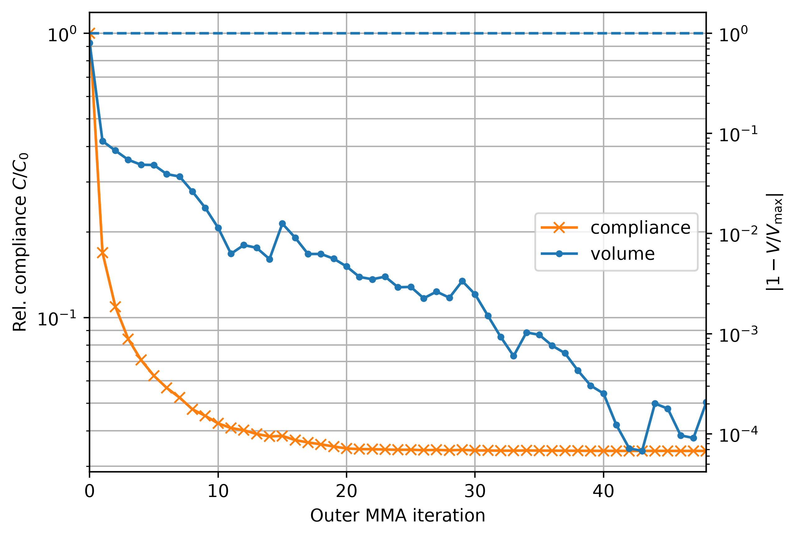
exit()Convergence of the optimisation, that is the compliance and the volume vs. outer MMA iteration are shown below. Compliance is measured relative to the initial compliance , which is compliance for the initial guess of . Volume is shown relative to the upper bound .
Source
matplotlib_inline.backend_inline.set_matplotlib_formats("png")
it = problem.tao.getIterationNumber()
comp = comp[:it]
volume = volume[:it]

fig, ax1 = plt.subplots(dpi=400)
ax1.set_xlim(0, it - 1)
ax1.set_xlabel("Outer MMA iteration")
ax1.set_ylabel("Rel. compliance $C / C_0$")
plt_compliance = ax1.plot(
    np.arange(0, it, dtype=int),
    comp / comp[0],
    color="tab:orange",
    marker="x",
)
ax1.set_yscale("log")
ax1.grid(True, which="both")

ax2 = ax1.twinx()
ax2.set_ylabel(r"$|1 - V / V_\text{max}|$")
plt_volume = ax2.plot(np.arange(0, it, dtype=int), np.abs(1 - volume / h[0].rhs), marker=".")
ax2.axhline(y=1, linestyle="--")
ax2.set_yscale("log")
ax1.legend(plt_compliance + plt_volume, ["compliance", "volume"], loc=7)

plt.show()
Figure 2:Convergence of compliance (relative to initial, orange) and volume constraint residual (blue) over MMA iterations.
The deformed final design (displacement scaled by )
Source
pixels = dolfiny.pyvista.pixels
plotter = pv.Plotter(window_size=[pixels, pixels // 2])
pv_grid.point_data[u.name] = u.x.array.reshape(-1, 3)
pv_grid.cell_data[s.name] = s.x.array
plotter.add_mesh(pv_grid.warp_by_vector(u.name, factor=5e3), color="black", line_width=1.5)
plotter.add_axes()
plotter.view_xy()
plotter.camera.elevation += 20
plotter.camera.zoom(2.0)
plotter.show()
plotter.close()
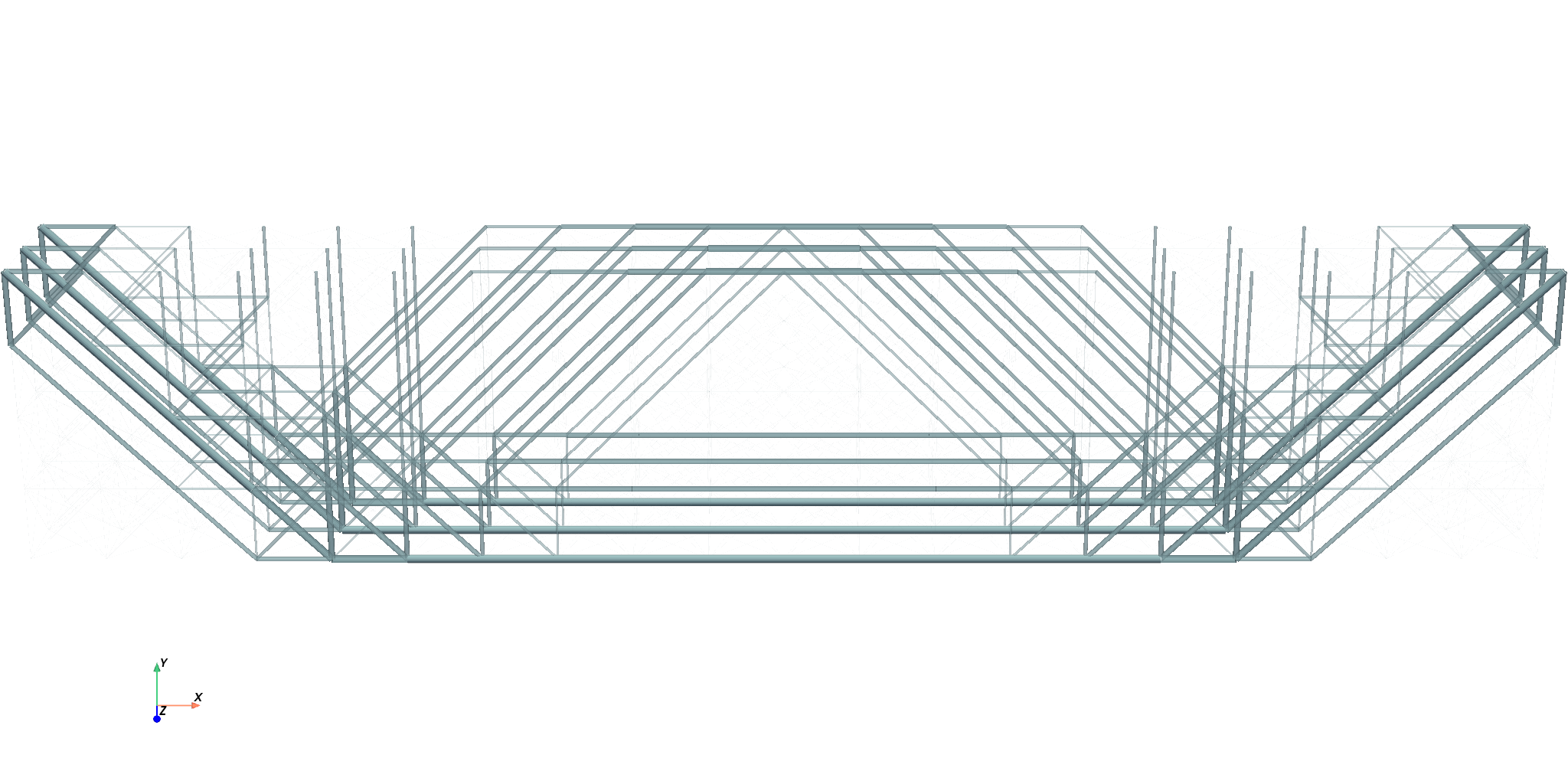
plotter.deep_clean()Figure 3:Deformed final truss design, displacement scaled by .

Visualisation of the optimised truss structure, each truss plotted corresponding to optimisation result (opacity of tubes according to ratio of maximal allowed cross sectional area). Radii are scaled by factor of 5, for visualisation purposes.
Source
plotter = pv.Plotter(window_size=[pixels, pixels // 2])

radius = np.sqrt(s.x.array / np.pi)
radius_max = np.sqrt(s_max / np.pi)
e_to_v = mesh.topology.connectivity(1, 0)
for e_idx in range(e_to_v.num_nodes):
    a, b = e_to_v.links(e_idx)
    plotter.add_mesh(
        pv.Tube(
            pointa=mesh.geometry.x[a],
            pointb=mesh.geometry.x[b],
            radius=radius[e_idx] * 5,
            capping=True,
        ),
        opacity=radius[e_idx] / radius_max,
    )
plotter.add_axes()
plotter.view_xy()
plotter.camera.elevation += 20
plotter.camera.zoom(2.0)
plotter.show()
plotter.close()
plotter.deep_clean()
Figure 4:Optimised truss structure rendered as tubes; opacity encodes the ratio of cross-sectional area to the maximum allowed area. Radii scaled by 5.
- Baratta, I. A., Dean, J. P., Dokken, J. S., Habera, M., Hale, J. S., Richardson, C. N., Rognes, M. E., Scroggs, M. W., Sime, N., & Wells, G. N. (2023). DOLFINx: The next generation FEniCS problem solving environment. Zenodo. 10.5281/zenodo.10447666
- Bleyer, J. (2024). Numerical tours of Computational Mechanics with FEniCSx (v0.2) [Computer software]. Zenodo. 10.5281/zenodo.13838486
- Christensen, P. W., & Klarbring, A. (2009). Sizing Stiffness Optimization of a Truss. In An Introduction to Structural Optimization (pp. 77–95). Springer Netherlands. 10.1007/978-1-4020-8666-3_5