This demo solves a three-dimensional hyperelastic torsion problem by expressing the constitutive law in terms of the eigenvalues of the Cauchy strain tensor. It demonstrates how to obtain those principal stretches symbolically and how to differentiate a strain-energy density written directly in terms of them.
In particular, this demo emphasizes:
symbolic principal-stretch extraction from the Cauchy strain tensor via
dolfiny.invariants.eigenstate,automatic differentiation of a strain energy written in spectral (eigenvalue) form with UFL,
dimensional analysis and non-dimensionalization via
dolfiny.units.
The task is to find a displacement field which solves the variational problem (principle of virtual displacements)
for all . Stress tensor (second Piola-Kirchhoff) is computed from bulk and shear strain energies which are defined for a compressible Neo-Hookean material Pence & Gou, 2014 as
with Cauchy strain tensor , deformation gradient and its derived invariants and and material parameters and .
For the hyperelastic material the strain energy is a potential for the stress tensor, i.e.
For isotropic strain energy functionals (which the Neo-Hookean model fulfils) we can write
for the three principal stresses (eigenvalues of the stress tensor ) and three principal stretches (eigenvalues of the strain tensor ) . Using the notion of principal stresses and stretches, the inner product contraction in the above variational problem simplifies to
The key point in the above is to express the strain energy functional purely in terms of principal stretches , which is achieved using
Principal stretches are available as symbolic closed-form expression of the primary unknown
displacement thanks to helper function dolfiny.invariants.eigenstate,
see Habera & Zilian (2021) for more detail.
Source
import argparse
import platform
import warnings

from mpi4py import MPI
from petsc4py import PETSc

import basix
import dolfinx
import ufl
from dolfinx import default_scalar_type as scalar

import numpy as np
import pyvista as pv
import sympy.physics.units as syu

import dolfiny
from dolfiny.expression import normalize
from dolfiny.units import Quantity

warnings.filterwarnings("error")

parser = argparse.ArgumentParser(
    description="Solid elasticity with classic or spectral formulation"
)
parser.add_argument(
    "--formulation",
    choices=["classic", "spectral"],
    default="spectral",
    help="Choose strain formulation: classic (Cauchy strain) or spectral (principal stretches)",
    required=False,
)
args, unknown = parser.parse_known_args()


def mesh_tube3d_gmshapi(
    name="tube3d",
    r=1.0,
    t=0.2,
    h=1.0,
    nr=30,
    nt=6,
    nh=10,
    x0=0.0,
    y0=0.0,
    z0=0.0,
    do_quads=False,
    order=1,
    msh_file=None,
    comm=MPI.COMM_WORLD,
):
    """
    Create mesh of 3d tube using the Python API of Gmsh.
    """
    tdim = 3  # target topological dimension

    # Perform Gmsh work only on rank = 0

    if comm.rank == 0:
        import gmsh

        # Initialise gmsh and set options
        gmsh.initialize()
        gmsh.option.setNumber("General.Terminal", 1)
        gmsh.option.set_number("General.NumThreads", 1)  # reproducibility

        if do_quads:
            gmsh.option.set_number("Mesh.Algorithm", 8)
            gmsh.option.set_number("Mesh.Algorithm3D", 10)
            # gmsh.option.set_number("Mesh.SubdivisionAlgorithm", 2)
        else:
            gmsh.option.set_number("Mesh.Algorithm", 5)
            gmsh.option.set_number("Mesh.Algorithm3D", 4)
            gmsh.option.set_number("Mesh.AlgorithmSwitchOnFailure", 6)

        # Add model under given name
        gmsh.model.add(name)

        # Create points and line
        p0 = gmsh.model.occ.add_point(x0 + r, y0, 0.0)
        p1 = gmsh.model.occ.add_point(x0 + r + t, y0, 0.0)
        l0 = gmsh.model.occ.add_line(p0, p1)
        s0 = gmsh.model.occ.revolve(
            [(1, l0)],
            x0,
            y0,
            z0,
            0,
            0,
            1,
            angle=+gmsh.pi,
            numElements=[nr],
            recombine=do_quads,
        )
        s1 = gmsh.model.occ.revolve(
            [(1, l0)],
            x0,
            y0,
            z0,
            0,
            0,
            1,
            angle=-gmsh.pi,
            numElements=[nr],
            recombine=do_quads,
        )
        ring, _ = gmsh.model.occ.fuse([s0[1]], [s1[1]])
        tube = gmsh.model.occ.extrude(ring, 0, 0, h, [nh], recombine=do_quads)  # noqa: F841

        # Synchronize
        gmsh.model.occ.synchronize()

        # Get model entities
        _points, _lines, surfaces, volumes = (gmsh.model.occ.get_entities(d) for d in [0, 1, 2, 3])
        boundaries = gmsh.model.get_boundary(volumes, oriented=False)  # noqa: F841

        # Assertions, problem-specific
        assert len(volumes) == 2

        # Helper
        def extract_tags(a):
            return list(ai[1] for ai in a)

        # Extract certain tags, problem-specific
        tag_subdomains_total = extract_tags(volumes)

        # Set geometrical identifiers (obtained by inspection)
        tag_interfaces_lower = extract_tags([surfaces[0], surfaces[1]])
        tag_interfaces_upper = extract_tags([surfaces[6], surfaces[9]])
        tag_interfaces_inner = extract_tags([surfaces[2], surfaces[7]])
        tag_interfaces_outer = extract_tags([surfaces[3], surfaces[8]])

        # Define physical groups for subdomains (! target tag > 0)
        domain = 1
        gmsh.model.add_physical_group(tdim, tag_subdomains_total, domain)
        gmsh.model.set_physical_name(tdim, domain, "domain")

        # Define physical groups for interfaces (! target tag > 0)
        surface_lower = 1
        gmsh.model.add_physical_group(tdim - 1, tag_interfaces_lower, surface_lower)
        gmsh.model.set_physical_name(tdim - 1, surface_lower, "surface_lower")
        surface_upper = 2
        gmsh.model.add_physical_group(tdim - 1, tag_interfaces_upper, surface_upper)
        gmsh.model.set_physical_name(tdim - 1, surface_upper, "surface_upper")
        surface_inner = 3
        gmsh.model.add_physical_group(tdim - 1, tag_interfaces_inner, surface_inner)
        gmsh.model.set_physical_name(tdim - 1, surface_inner, "surface_inner")
        surface_outer = 4
        gmsh.model.add_physical_group(tdim - 1, tag_interfaces_outer, surface_outer)
        gmsh.model.set_physical_name(tdim - 1, surface_outer, "surface_outer")

        # Set refinement in radial direction
        gmsh.model.mesh.setTransfiniteCurve(l0, numNodes=nt)

        # Generate the mesh
        gmsh.model.mesh.generate()

        # Set geometric order of mesh cells
        gmsh.model.mesh.setOrder(order)

        # Optional: Write msh file
        if msh_file is not None:
            gmsh.write(msh_file)

    return gmsh.model if comm.rank == 0 else None, tdim


class Xdmf3Reader(pv.XdmfReader):
    _vtk_module_name = "vtkIOXdmf3"
    _vtk_class_name = "vtkXdmf3Reader"


def plot_tube3d_pyvista(u, s, comm=MPI.COMM_WORLD):
    if comm.rank > 0:
        return

    grid = pv.UnstructuredGrid(*dolfinx.plot.vtk_mesh(u.function_space))

    plotter = pv.Plotter(off_screen=True, theme=dolfiny.pyvista.theme)
    plotter.add_axes()
    plotter.enable_parallel_projection()

    grid.point_data["u"] = u.x.array.reshape(-1, 3)
    grid.point_data["von_mises"] = s.x.array / 1e6  # to MPa

    grid_warped = grid.warp_by_vector("u", factor=1.0)

    if not grid.get_cell(0).is_linear:
        levels = 4
    else:
        levels = 0

    s = plotter.add_mesh(
        grid_warped.extract_surface(nonlinear_subdivision=levels, algorithm="dataset_surface"),
        scalars="von_mises",
        scalar_bar_args={"title": "von Mises stress [MPa]"},
        n_colors=10,
    )

    s.mapper.scalar_range = [0.0, 0.6]

    plotter.add_mesh(
        grid_warped.separate_cells()
        .extract_surface(nonlinear_subdivision=levels, algorithm="dataset_surface")
        .extract_feature_edges(),
        style="wireframe",
        color="black",
        line_width=dolfiny.pyvista.pixels // 1000,
        render_lines_as_tubes=True,
    )

    plotter.show_axes()
    plotter.show()
    plotter.close()
    plotter.deep_clean()
This demo is parametrised by the choice of formulation: “classic” or “spectral”. The classic formulation uses the main invariants of the Cauchy strain tensor, while the spectral formulation writes the strain energy directly in terms of the principal stretches.
Source
print(f"Arguments: {args}")Arguments: Namespace(formulation='spectral')
Meshing, boundary tagging and function spaces definition
Mesh in this example is a tube with radius , thickness and height . It is tesselated using 27 node quadratic hexahedral elements.
Bottom of the tube is marked as “surface_lower” and top is marked as “surface_upper”.
Source
name = f"solid_elasticity_{args.formulation}"
comm = MPI.COMM_WORLD

# Geometry and mesh parameters
r, t, h = 0.4, 0.1, 1
nr, nt, nh = 16, 5, 8

# Create the regular mesh of a tube with given dimensions
gmsh_model, tdim = mesh_tube3d_gmshapi(name, r, t, h, nr, nt, nh, do_quads=True, order=2)

# Get mesh and meshtags
mesh_data = dolfinx.io.gmsh.model_to_mesh(gmsh_model, comm, rank=0)
mesh = mesh_data.mesh

# Define shorthands for labelled tags
surface_lower = mesh_data.physical_groups["surface_lower"].tag
surface_upper = mesh_data.physical_groups["surface_upper"].tag
Output
Info    : Meshing 1D...
Info    : [  0%] Meshing curve 1 (Line)
Info    : [ 10%] Meshing curve 2 (Extruded)
Info    : [ 20%] Meshing curve 3 (Extruded)
Info    : [ 20%] Meshing curve 4 (Extruded)
Info    : [ 30%] Meshing curve 5 (Extruded)
Info    : [ 40%] Meshing curve 6 (Extruded)
Info    : [ 40%] Meshing curve 7 (Extruded)
Info    : [ 50%] Meshing curve 8 (Extruded)
Info    : [ 60%] Meshing curve 9 (Extruded)
Info    : [ 60%] Meshing curve 10 (Extruded)
Info    : [ 70%] Meshing curve 11 (Extruded)
Info    : [ 70%] Meshing curve 12 (Extruded)
Info    : [ 80%] Meshing curve 13 (Extruded)
Info    : [ 90%] Meshing curve 14 (Extruded)
Info    : [ 90%] Meshing curve 15 (Extruded)
Info    : [100%] Meshing curve 16 (Extruded)
Info    : Done meshing 1D (Wall 0.000161406s, CPU 0.00041s)
Info    : Meshing 2D...
Info    : [  0%] Meshing surface 1 (Extruded)
Info    : [ 20%] Meshing surface 2 (Extruded)
Info    : [ 30%] Meshing surface 3 (Extruded)
Info    : [ 40%] Meshing surface 4 (Extruded)
Info    : [ 50%] Meshing surface 5 (Extruded)
Info    : [ 60%] Meshing surface 6 (Extruded)
Info    : [ 70%] Meshing surface 7 (Extruded)
Info    : [ 80%] Meshing surface 8 (Extruded)
Info    : [ 90%] Meshing surface 9 (Extruded)
Info    : [100%] Meshing surface 10 (Extruded)
Info    : Done meshing 2D (Wall 0.00163506s, CPU 0.001378s)
Info    : Meshing 3D...
Info    : Meshing volume 1 (Extruded)
Info    : Meshing volume 2 (Extruded)
Info    : Done meshing 3D (Wall 0.00281224s, CPU 0.002808s)
Info    : 1440 nodes 2040 elements
Info    : Meshing order 2 (curvilinear on)...
Info    : [  0%] Meshing curve 1 order 2
Info    : [ 10%] Meshing curve 2 order 2
Info    : [ 10%] Meshing curve 3 order 2
Info    : [ 20%] Meshing curve 4 order 2
Info    : [ 20%] Meshing curve 5 order 2
Info    : [ 20%] Meshing curve 6 order 2
Info    : [ 30%] Meshing curve 7 order 2
Info    : [ 30%] Meshing curve 8 order 2
Info    : [ 30%] Meshing curve 9 order 2
Info    : [ 40%] Meshing curve 10 order 2
Info    : [ 40%] Meshing curve 11 order 2
Info    : [ 40%] Meshing curve 12 order 2
Info    : [ 50%] Meshing curve 13 order 2
Info    : [ 50%] Meshing curve 14 order 2
Info    : [ 60%] Meshing curve 15 order 2
Info    : [ 60%] Meshing curve 16 order 2
Info    : [ 60%] Meshing surface 1 order 2
Info    : [ 70%] Meshing surface 2 order 2
Info    : [ 70%] Meshing surface 3 order 2
Info    : [ 70%] Meshing surface 4 order 2
Info    : [ 80%] Meshing surface 5 order 2
Info    : [ 80%] Meshing surface 6 order 2
Info    : [ 80%] Meshing surface 7 order 2
Info    : [ 90%] Meshing surface 8 order 2
Info    : [ 90%] Meshing surface 9 order 2
Info    : [ 90%] Meshing surface 10 order 2
Info    : [100%] Meshing volume 1 order 2
Info    : [100%] Meshing volume 2 order 2
Info    : Done meshing order 2 (Wall 0.0176834s, CPU 0.017684s)
Quadrature rule is limited to the 4th degree for performance reasons. The symbolic expressions resulting from the eigenvalues of the Cauchy strain tensor are rather involved so the time to assemble the forms increases.
Function space discretisation is based on vector-valued isoparametric continuous Lagrange element with three components - since we model the displacement in three dimensions.
Source
dx = ufl.Measure(
    "dx", domain=mesh, subdomain_data=mesh_data.cell_tags, metadata={"quadrature_degree": 4}
)
ds = ufl.Measure(
    "ds", domain=mesh, subdomain_data=mesh_data.facet_tags, metadata={"quadrature_degree": 4}
)

Ue = basix.ufl.element("P", mesh.basix_cell(), 2, shape=(mesh.geometry.dim,))
Uf = dolfinx.fem.functionspace(mesh, Ue)

# Define functions
u = dolfinx.fem.Function(Uf, name="u")
u_ = dolfinx.fem.Function(Uf, name="u_")  # boundary conditions

δm = ufl.TestFunctions(ufl.MixedFunctionSpace(Uf))
(δu,) = δm

# Define state as (ordered) list of functions
m = [u]

# Functions for output / visualisation
vorder = mesh.geometry.cmaps[0].degree
uo = dolfinx.fem.Function(dolfinx.fem.functionspace(mesh, ("P", vorder, (3,))), name="u")
so = dolfinx.fem.Function(dolfinx.fem.functionspace(mesh, ("P", vorder)), name="s")  # for output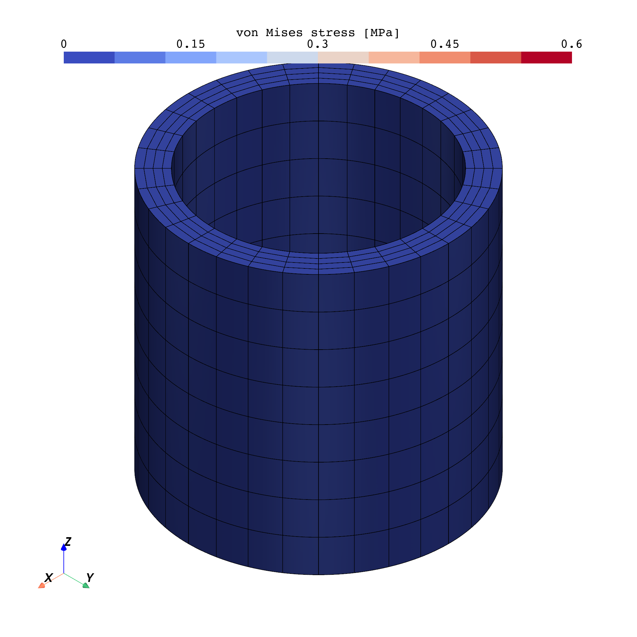
Material parameters with units
There are four dimensional quantities in the problem:
| Parameter | Value | Description |
|---|---|---|
| reference length scale | ||
| load scale | ||
| shear modulus | ||
| bulk modulus |
derived from Poisson ratio , Lamé coefficient and Young’s modulus .
We can execute the Buckingham Pi analysis which shows overview of the dimensional quantities and derives a set of dimensionless numbers. In this examaple we arrive at two dimensionless numbers:
bulk-to-shear ratio and
loading factor .
Source
nu = 0.4
E = Quantity(mesh, 1, syu.mega * syu.pascal, "E")
λ = Quantity(mesh, E.scale * nu / ((1 + nu) * (1 - 2 * nu)), syu.mega * syu.pascal, "λ")

μ = Quantity(mesh, E.scale / (2 * (1 + nu)), syu.mega * syu.pascal, "μ")
κ = Quantity(mesh, λ.scale + 2 / 3 * μ.scale, syu.mega * syu.pascal, "κ")

l_ref = Quantity(mesh, 0.1, syu.meter, "l_ref")
t_ref = Quantity(mesh, 0.2, syu.mega * syu.pascal, "t_ref")
u_ref = Quantity(mesh, 1.0, syu.meter, "u_ref")

quantities = [μ, κ, l_ref, t_ref, u_ref]
# quantities = [μ, κ, l_ref, t_ref]
if comm.rank == 0:
    dolfiny.units.buckingham_pi_analysis(quantities)
==================================================
Buckingham Pi Analysis
==================================================
Symbol | Expression | Value (in base units)
-------+-----------------+------------------------------------
μ | 3.571e+5*pascal | 3.571e+5*kilogram/(meter*second**2)
κ | 1.667e+6*pascal | 1.667e+6*kilogram/(meter*second**2)
l_ref | 0.1*meter | 0.1*meter
t_ref | 2.0e+5*pascal | 2.0e+5*kilogram/(meter*second**2)
u_ref | 1.0*meter | 1.0*meter
Dimension matrix (7 x 5):
Dimension | μ | κ | l_ref | t_ref | u_ref
--------------------+----+----+-------+-------+------
amount_of_substance | 0 | 0 | 0 | 0 | 0
current | 0 | 0 | 0 | 0 | 0
length | -1 | -1 | 1 | -1 | 1
luminous_intensity | 0 | 0 | 0 | 0 | 0
mass | 1 | 1 | 0 | 1 | 0
temperature | 0 | 0 | 0 | 0 | 0
time | -2 | -2 | 0 | -2 | 0
Dimensionless groups (3):
Group | Expression | Value
------+-------------+------
Pi_1 | κ/μ | 4.67
Pi_2 | t_ref/μ | 0.56
Pi_3 | u_ref/l_ref | 10
==================================================
Weak form
Source
F = ufl.Identity(3) + ufl.grad(u)

# Strain measure: Cauchy strain tensor
C = F.T * F
C = ufl.variable(C)


def strain_energy_bulk(i1, i2, i3):
    J = ufl.sqrt(i3)
    return κ / 2 * (J - 1) ** 2


def strain_energy_shear(i1, i2, i3):
    J = ufl.sqrt(i3)
    return μ / 2 * (i1 - 3 - 2 * ufl.ln(J))


def von_mises_stress(S):
    return ufl.sqrt(3 / 2 * ufl.inner(ufl.dev(S), ufl.dev(S)))


# Formulation-specific strain measures
if args.formulation == "spectral":
    c, _ = dolfiny.invariants.eigenstate(C)
    c = ufl.as_vector(c)
    c = ufl.variable(c)

    # Reconstruct the principal invariants from the principal stretches
    i1, i2, i3 = c[0] + c[1] + c[2], c[0] * c[1] + c[1] * c[2] + c[0] * c[2], c[0] * c[1] * c[2]

    δC = ufl.derivative(c, m, δm)
    S_bulk = 2 * ufl.diff(strain_energy_bulk(i1, i2, i3), c)
    S_shear = 2 * ufl.diff(strain_energy_shear(i1, i2, i3), c)
    S = S_bulk + S_shear

    svm = von_mises_stress(ufl.diag(S))
elif args.formulation == "classic":
    δC = ufl.derivative(C, m, δm)

    i1, i2, i3 = dolfiny.invariants.invariants_principal(C)

    S_bulk = 2 * ufl.diff(strain_energy_bulk(i1, i2, i3), C)
    S_shear = 2 * ufl.diff(strain_energy_shear(i1, i2, i3), C)
    S = S_bulk + S_shear

    svm = von_mises_stress(S)
else:
    raise RuntimeError(f"Unknown formulation '{args.formulation}'")
Boundary traction is created to represent rotational vector field in the shifted -plane which is scaled with the reference load scale . We first compute radial vector field in the shifted -plane
which we normalize and cross product with the unit vector ,
A load factor is increased from 0 to 1 during the loading procedure.
Source
x0 = ufl.SpatialCoordinate(mesh)
load_factor = dolfinx.fem.Constant(mesh, scalar(0.0))
ez = ufl.as_vector([0.0, 0.0, 1.0])
d = normalize(x0 - l_ref * h * ez)
t = ufl.cross(d, ez) * load_factor

mapping = {
    mesh.ufl_domain(): l_ref,
    u: l_ref * u,
    δu: l_ref * δu,
}

terms = {
    "bulk": -1 / 2 * ufl.inner(δC, S_bulk) * dx,
    "shear": -1 / 2 * ufl.inner(δC, S_shear) * dx,
    "external": ufl.inner(δu, t_ref * t) * ds(surface_upper),
}
factorized = dolfiny.units.factorize(terms, quantities, mode="factorize", mapping=mapping)
assert isinstance(factorized, dict)

dimsys = syu.si.SI.get_dimension_system()
assert dimsys.equivalent_dims(
    dolfiny.units.get_dimension(terms["bulk"], quantities, mapping),
    syu.energy,
)
assert dimsys.equivalent_dims(
    dolfiny.units.get_dimension(strain_energy_bulk(i1, i2, i3), quantities, mapping),
    syu.energy * syu.length**-3,
)
assert dimsys.equivalent_dims(
    dolfiny.units.get_dimension(S_shear, quantities, mapping),
    syu.pressure,
)

reference_term = "bulk"
ref_factor = factorized[reference_term].factor

normalized = dolfiny.units.normalize(factorized, reference_term, quantities)
form = sum(normalized.values(), ufl.form.Zero())

# Overall form (as list of forms)
forms = ufl.extract_blocks(form)  # type: ignore
==================================================
Terms after normalization with "bulk"
==================================================
Reference factor from 'bulk':
Term | Factor | Value (in base units)
-----+------------+-----------------------------------
bulk | l_ref**3*κ | 1667.0*kilogram*meter**2/second**2
Term | Factor | Value (in base units)
---------+---------+----------------------
bulk | 1 | 1.000
shear | μ/κ | 0.2143
external | t_ref/κ | 0.1200
==================================================
The problem solved leads to symmetric positive definite system on the algebraic level. We choose to solve it using MUMPS Cholesky solver for general symmetric matrices. We explicitly numerical pivoting by setting CNTL(1) = 0.
The nonlinear SNES solver is configured to use Newton line search with no (basic) line search.
Source
opts = PETSc.Options(name)  # type: ignore[attr-defined]
opts["snes_type"] = "newtonls"
opts["snes_linesearch_type"] = "basic"
opts["snes_rtol"] = 1.0e-08
opts["snes_max_it"] = 10
opts["ksp_type"] = "preonly"
opts["pc_type"] = "cholesky"
opts["pc_factor_mat_solver_type"] = "mumps"
opts["mat_mumps_cntl_1"] = 0.0 # Disable relative pivoting thresholdSource
# FFCx options (formulation-specific)
if args.formulation == "spectral":
    # ARM64-specific optimizations for spectral formulation
    flags = [
        "-fno-schedule-insns",
        "-fno-schedule-insns2",
    ]
    if platform.system() != "Darwin":
        flags.append("-fdisable-rtl-combine")
    jit_options = dict(cffi_extra_compile_args=flags)
else:
    # Standard options for classic formulation
    jit_options = dict(cffi_extra_compile_args=["-g0"])

# Create nonlinear problem: SNES
problem = dolfiny.snesproblem.SNESProblem(forms, m, prefix=name, jit_options=jit_options)

# Identify dofs of function spaces associated with tagged interfaces/boundaries
b_dofs_Uf = dolfiny.mesh.locate_dofs_topological(Uf, mesh_data.facet_tags, surface_lower)

# Set/update boundary conditions
problem.bcs = [
    dolfinx.fem.dirichletbc(u_, b_dofs_Uf),  # u lower face
]

# Apply external force via load stepping
for lf in np.linspace(0.0, 1.0, 10 + 1)[1:]:
    # Set load factor
    load_factor.value = lf
    dolfiny.utils.pprint(f"\n*** Load factor = {lf:.4f} ({args.formulation} formulation) \n")

    # Solve nonlinear problem
    problem.solve()

    # Assert convergence of nonlinear solver
    problem.status(verbose=True, error_on_failure=True)

    # Assert symmetry of operator
    assert dolfiny.la.is_symmetric(problem.J)

# Interpolate for output purposes
dolfiny.interpolation.interpolate(u, uo)
dolfiny.interpolation.interpolate(svm, so)

# Write results to file
with dolfiny.io.XDMFFile(comm, f"{name}.xdmf", "w") as ofile:
    ofile.write_mesh_meshtags(mesh)
    ofile.write_function(uo)
    ofile.write_function(so)
Output
cc1: note: disable pass rtl-combine for functions in the range of [0, 4294967295]
cc1: note: disable pass rtl-combine for functions in the range of [0, 4294967295]
libffcx_forms_f1340e0b607f39bfd374f7667e72ff9b894d7d1b.c: In function ‘tabulate_tensor_integral_edb6f5445b933a32a5723dc32c99e27f5c6cdfc2_hexahedron’:
libffcx_forms_f1340e0b607f39bfd374f7667e72ff9b894d7d1b.c:598:6: note: variable tracking size limit exceeded with ‘-fvar-tracking-assignments’, retrying without
  598 | void tabulate_tensor_integral_edb6f5445b933a32a5723dc32c99e27f5c6cdfc2_hexahedron(double* restrict A,
      |      ^~~~~~~~~~~~~~~~~~~~~~~~~~~~~~~~~~~~~~~~~~~~~~~~~~~~~~~~~~~~~~~~~~~~~~~~~~~~
*** Load factor = 0.1000 (spectral formulation)
# SNES iteration 0
# sub 0 [ 29k] |x|=0.000e+00 |dx|=0.000e+00 |r|=1.653e-04 (u)
# all |x|=0.000e+00 |dx|=0.000e+00 |r|=1.653e-04
# SNES iteration 0, KSP iteration 0 |r|=1.653e-04
# SNES iteration 0, KSP iteration 1 |r|=2.536e-16
# SNES iteration 1
# sub 0 [ 29k] |x|=3.355e+00 |dx|=3.355e+00 |r|=1.258e-03 (u)
# all |x|=3.355e+00 |dx|=3.355e+00 |r|=1.258e-03
# SNES iteration 1, KSP iteration 0 |r|=1.258e-03
# SNES iteration 1, KSP iteration 1 |r|=2.395e-17
# SNES iteration 2
# sub 0 [ 29k] |x|=3.256e+00 |dx|=1.644e-01 |r|=2.691e-05 (u)
# all |x|=3.256e+00 |dx|=1.644e-01 |r|=2.691e-05
# SNES iteration 2, KSP iteration 0 |r|=2.691e-05
# SNES iteration 2, KSP iteration 1 |r|=5.191e-18
# SNES iteration 3
# sub 0 [ 29k] |x|=3.253e+00 |dx|=4.947e-02 |r|=9.646e-06 (u)
# all |x|=3.253e+00 |dx|=4.947e-02 |r|=9.646e-06
# SNES iteration 3, KSP iteration 0 |r|=9.646e-06
# SNES iteration 3, KSP iteration 1 |r|=9.691e-20
# SNES iteration 4
# sub 0 [ 29k] |x|=3.253e+00 |dx|=9.594e-04 |r|=4.645e-09 (u)
# all |x|=3.253e+00 |dx|=9.594e-04 |r|=4.645e-09
# SNES iteration 4, KSP iteration 0 |r|=4.645e-09
# SNES iteration 4, KSP iteration 1 |r|=6.974e-22
# SNES iteration 5 success = CONVERGED_FNORM_RELATIVE
# sub 0 [ 29k] |x|=3.253e+00 |dx|=6.808e-06 |r|=2.275e-13 (u)
# all |x|=3.253e+00 |dx|=6.808e-06 |r|=2.275e-13
absolute asymmetry measure = 3.811e-16
relative asymmetry measure = 9.743e-17
*** Load factor = 0.2000 (spectral formulation)
# SNES iteration 0
# sub 0 [ 29k] |x|=3.253e+00 |dx|=6.808e-06 |r|=1.653e-04 (u)
# all |x|=3.253e+00 |dx|=6.808e-06 |r|=1.653e-04
# SNES iteration 0, KSP iteration 0 |r|=1.653e-04
# SNES iteration 0, KSP iteration 1 |r|=2.586e-16
# SNES iteration 1
# sub 0 [ 29k] |x|=6.563e+00 |dx|=3.312e+00 |r|=1.472e-03 (u)
# all |x|=6.563e+00 |dx|=3.312e+00 |r|=1.472e-03
# SNES iteration 1, KSP iteration 0 |r|=1.472e-03
# SNES iteration 1, KSP iteration 1 |r|=2.180e-17
# SNES iteration 2
# sub 0 [ 29k] |x|=6.615e+00 |dx|=1.439e-01 |r|=2.808e-05 (u)
# all |x|=6.615e+00 |dx|=1.439e-01 |r|=2.808e-05
# SNES iteration 2, KSP iteration 0 |r|=2.808e-05
# SNES iteration 2, KSP iteration 1 |r|=7.638e-18
# SNES iteration 3
# sub 0 [ 29k] |x|=6.664e+00 |dx|=7.284e-02 |r|=1.491e-05 (u)
# all |x|=6.664e+00 |dx|=7.284e-02 |r|=1.491e-05
# SNES iteration 3, KSP iteration 0 |r|=1.491e-05
# SNES iteration 3, KSP iteration 1 |r|=1.367e-19
# SNES iteration 4
# sub 0 [ 29k] |x|=6.665e+00 |dx|=1.429e-03 |r|=8.404e-09 (u)
# all |x|=6.665e+00 |dx|=1.429e-03 |r|=8.404e-09
# SNES iteration 4, KSP iteration 0 |r|=8.404e-09
# SNES iteration 4, KSP iteration 1 |r|=1.472e-21
# SNES iteration 5 success = CONVERGED_FNORM_RELATIVE
# sub 0 [ 29k] |x|=6.665e+00 |dx|=1.503e-05 |r|=9.099e-13 (u)
# all |x|=6.665e+00 |dx|=1.503e-05 |r|=9.099e-13
absolute asymmetry measure = 3.808e-16
relative asymmetry measure = 9.227e-17
*** Load factor = 0.3000 (spectral formulation)
# SNES iteration 0
# sub 0 [ 29k] |x|=6.665e+00 |dx|=1.503e-05 |r|=1.653e-04 (u)
# all |x|=6.665e+00 |dx|=1.503e-05 |r|=1.653e-04
# SNES iteration 0, KSP iteration 0 |r|=1.653e-04
# SNES iteration 0, KSP iteration 1 |r|=2.838e-16
# SNES iteration 1
# sub 0 [ 29k] |x|=1.020e+01 |dx|=3.547e+00 |r|=2.479e-03 (u)
# all |x|=1.020e+01 |dx|=3.547e+00 |r|=2.479e-03
# SNES iteration 1, KSP iteration 0 |r|=2.479e-03
# SNES iteration 1, KSP iteration 1 |r|=2.170e-17
# SNES iteration 2
# sub 0 [ 29k] |x|=1.026e+01 |dx|=1.653e-01 |r|=4.638e-05 (u)
# all |x|=1.026e+01 |dx|=1.653e-01 |r|=4.638e-05
# SNES iteration 2, KSP iteration 0 |r|=4.638e-05
# SNES iteration 2, KSP iteration 1 |r|=9.216e-18
# SNES iteration 3
# sub 0 [ 29k] |x|=1.033e+01 |dx|=9.295e-02 |r|=2.039e-05 (u)
# all |x|=1.033e+01 |dx|=9.295e-02 |r|=2.039e-05
# SNES iteration 3, KSP iteration 0 |r|=2.039e-05
# SNES iteration 3, KSP iteration 1 |r|=3.234e-19
# SNES iteration 4
# sub 0 [ 29k] |x|=1.033e+01 |dx|=3.342e-03 |r|=3.430e-08 (u)
# all |x|=1.033e+01 |dx|=3.342e-03 |r|=3.430e-08
# SNES iteration 4, KSP iteration 0 |r|=3.430e-08
# SNES iteration 4, KSP iteration 1 |r|=4.817e-21
# SNES iteration 5
# sub 0 [ 29k] |x|=1.033e+01 |dx|=5.170e-05 |r|=8.867e-12 (u)
# all |x|=1.033e+01 |dx|=5.170e-05 |r|=8.867e-12
# SNES iteration 5, KSP iteration 0 |r|=8.867e-12
# SNES iteration 5, KSP iteration 1 |r|=1.264e-25
# SNES iteration 6 success = CONVERGED_FNORM_RELATIVE
# sub 0 [ 29k] |x|=1.033e+01 |dx|=1.307e-09 |r|=3.127e-16 (u)
# all |x|=1.033e+01 |dx|=1.307e-09 |r|=3.127e-16
absolute asymmetry measure = 3.953e-16
relative asymmetry measure = 8.838e-17
*** Load factor = 0.4000 (spectral formulation)
# SNES iteration 0
# sub 0 [ 29k] |x|=1.033e+01 |dx|=1.307e-09 |r|=1.653e-04 (u)
# all |x|=1.033e+01 |dx|=1.307e-09 |r|=1.653e-04
# SNES iteration 0, KSP iteration 0 |r|=1.653e-04
# SNES iteration 0, KSP iteration 1 |r|=3.137e-16
# SNES iteration 1
# sub 0 [ 29k] |x|=1.413e+01 |dx|=3.827e+00 |r|=4.048e-03 (u)
# all |x|=1.413e+01 |dx|=3.827e+00 |r|=4.048e-03
# SNES iteration 1, KSP iteration 0 |r|=4.048e-03
# SNES iteration 1, KSP iteration 1 |r|=2.109e-17
# SNES iteration 2
# sub 0 [ 29k] |x|=1.415e+01 |dx|=1.850e-01 |r|=1.075e-04 (u)
# all |x|=1.415e+01 |dx|=1.850e-01 |r|=1.075e-04
# SNES iteration 2, KSP iteration 0 |r|=1.075e-04
# SNES iteration 2, KSP iteration 1 |r|=6.190e-18
# SNES iteration 3
# sub 0 [ 29k] |x|=1.419e+01 |dx|=5.544e-02 |r|=7.397e-06 (u)
# all |x|=1.419e+01 |dx|=5.544e-02 |r|=7.397e-06
# SNES iteration 3, KSP iteration 0 |r|=7.397e-06
# SNES iteration 3, KSP iteration 1 |r|=4.825e-19
# SNES iteration 4
# sub 0 [ 29k] |x|=1.419e+01 |dx|=4.906e-03 |r|=6.294e-08 (u)
# all |x|=1.419e+01 |dx|=4.906e-03 |r|=6.294e-08
# SNES iteration 4, KSP iteration 0 |r|=6.294e-08
# SNES iteration 4, KSP iteration 1 |r|=2.619e-21
# SNES iteration 5
# sub 0 [ 29k] |x|=1.419e+01 |dx|=2.603e-05 |r|=1.940e-12 (u)
# all |x|=1.419e+01 |dx|=2.603e-05 |r|=1.940e-12
# SNES iteration 5, KSP iteration 0 |r|=1.940e-12
# SNES iteration 5, KSP iteration 1 |r|=1.260e-25
# SNES iteration 6 success = CONVERGED_FNORM_RELATIVE
# sub 0 [ 29k] |x|=1.419e+01 |dx|=1.247e-09 |r|=4.237e-16 (u)
# all |x|=1.419e+01 |dx|=1.247e-09 |r|=4.237e-16
absolute asymmetry measure = 4.131e-16
relative asymmetry measure = 8.750e-17
*** Load factor = 0.5000 (spectral formulation)
# SNES iteration 0
# sub 0 [ 29k] |x|=1.419e+01 |dx|=1.247e-09 |r|=1.653e-04 (u)
# all |x|=1.419e+01 |dx|=1.247e-09 |r|=1.653e-04
# SNES iteration 0, KSP iteration 0 |r|=1.653e-04
# SNES iteration 0, KSP iteration 1 |r|=3.350e-16
# SNES iteration 1
# sub 0 [ 29k] |x|=1.808e+01 |dx|=3.946e+00 |r|=5.126e-03 (u)
# all |x|=1.808e+01 |dx|=3.946e+00 |r|=5.126e-03
# SNES iteration 1, KSP iteration 0 |r|=5.126e-03
# SNES iteration 1, KSP iteration 1 |r|=2.157e-17
# SNES iteration 2
# sub 0 [ 29k] |x|=1.804e+01 |dx|=1.959e-01 |r|=1.674e-04 (u)
# all |x|=1.804e+01 |dx|=1.959e-01 |r|=1.674e-04
# SNES iteration 2, KSP iteration 0 |r|=1.674e-04
# SNES iteration 2, KSP iteration 1 |r|=8.249e-18
# SNES iteration 3
# sub 0 [ 29k] |x|=1.799e+01 |dx|=5.355e-02 |r|=1.606e-06 (u)
# all |x|=1.799e+01 |dx|=5.355e-02 |r|=1.606e-06
# SNES iteration 3, KSP iteration 0 |r|=1.606e-06
# SNES iteration 3, KSP iteration 1 |r|=2.335e-19
# SNES iteration 4
# sub 0 [ 29k] |x|=1.799e+01 |dx|=2.289e-03 |r|=1.538e-08 (u)
# all |x|=1.799e+01 |dx|=2.289e-03 |r|=1.538e-08
# SNES iteration 4, KSP iteration 0 |r|=1.538e-08
# SNES iteration 4, KSP iteration 1 |r|=2.170e-22
# SNES iteration 5 success = CONVERGED_FNORM_RELATIVE
# sub 0 [ 29k] |x|=1.799e+01 |dx|=2.299e-06 |r|=2.195e-14 (u)
# all |x|=1.799e+01 |dx|=2.299e-06 |r|=2.195e-14
absolute asymmetry measure = 5.605e-16
relative asymmetry measure = 1.175e-16
*** Load factor = 0.6000 (spectral formulation)
# SNES iteration 0
# sub 0 [ 29k] |x|=1.799e+01 |dx|=2.299e-06 |r|=1.653e-04 (u)
# all |x|=1.799e+01 |dx|=2.299e-06 |r|=1.653e-04
# SNES iteration 0, KSP iteration 0 |r|=1.653e-04
# SNES iteration 0, KSP iteration 1 |r|=3.236e-16
# SNES iteration 1
# sub 0 [ 29k] |x|=2.169e+01 |dx|=3.782e+00 |r|=4.790e-03 (u)
# all |x|=2.169e+01 |dx|=3.782e+00 |r|=4.790e-03
# SNES iteration 1, KSP iteration 0 |r|=4.790e-03
# SNES iteration 1, KSP iteration 1 |r|=2.155e-17
# SNES iteration 2
# sub 0 [ 29k] |x|=2.160e+01 |dx|=1.899e-01 |r|=1.478e-04 (u)
# all |x|=2.160e+01 |dx|=1.899e-01 |r|=1.478e-04
# SNES iteration 2, KSP iteration 0 |r|=1.478e-04
# SNES iteration 2, KSP iteration 1 |r|=1.002e-17
# SNES iteration 3
# sub 0 [ 29k] |x|=2.150e+01 |dx|=9.993e-02 |r|=1.152e-05 (u)
# all |x|=2.150e+01 |dx|=9.993e-02 |r|=1.152e-05
# SNES iteration 3, KSP iteration 0 |r|=1.152e-05
# SNES iteration 3, KSP iteration 1 |r|=7.499e-19
# SNES iteration 4
# sub 0 [ 29k] |x|=2.150e+01 |dx|=6.437e-03 |r|=1.124e-07 (u)
# all |x|=2.150e+01 |dx|=6.437e-03 |r|=1.124e-07
# SNES iteration 4, KSP iteration 0 |r|=1.124e-07
# SNES iteration 4, KSP iteration 1 |r|=5.182e-21
# SNES iteration 5
# sub 0 [ 29k] |x|=2.150e+01 |dx|=4.364e-05 |r|=6.216e-12 (u)
# all |x|=2.150e+01 |dx|=4.364e-05 |r|=6.216e-12
# SNES iteration 5, KSP iteration 0 |r|=6.216e-12
# SNES iteration 5, KSP iteration 1 |r|=3.559e-25
# SNES iteration 6 success = CONVERGED_FNORM_RELATIVE
# sub 0 [ 29k] |x|=2.150e+01 |dx|=3.058e-09 |r|=6.032e-16 (u)
# all |x|=2.150e+01 |dx|=3.058e-09 |r|=6.032e-16
absolute asymmetry measure = 4.820e-16
relative asymmetry measure = 8.183e-17
*** Load factor = 0.7000 (spectral formulation)
# SNES iteration 0
# sub 0 [ 29k] |x|=2.150e+01 |dx|=3.058e-09 |r|=1.653e-04 (u)
# all |x|=2.150e+01 |dx|=3.058e-09 |r|=1.653e-04
# SNES iteration 0, KSP iteration 0 |r|=1.653e-04
# SNES iteration 0, KSP iteration 1 |r|=3.069e-16
# SNES iteration 1
# sub 0 [ 29k] |x|=2.483e+01 |dx|=3.441e+00 |r|=3.670e-03 (u)
# all |x|=2.483e+01 |dx|=3.441e+00 |r|=3.670e-03
# SNES iteration 1, KSP iteration 0 |r|=3.670e-03
# SNES iteration 1, KSP iteration 1 |r|=1.897e-17
# SNES iteration 2
# sub 0 [ 29k] |x|=2.471e+01 |dx|=1.720e-01 |r|=9.135e-05 (u)
# all |x|=2.471e+01 |dx|=1.720e-01 |r|=9.135e-05
# SNES iteration 2, KSP iteration 0 |r|=9.135e-05
# SNES iteration 2, KSP iteration 1 |r|=1.076e-17
# SNES iteration 3
# sub 0 [ 29k] |x|=2.462e+01 |dx|=9.648e-02 |r|=1.270e-05 (u)
# all |x|=2.462e+01 |dx|=9.648e-02 |r|=1.270e-05
# SNES iteration 3, KSP iteration 0 |r|=1.270e-05
# SNES iteration 3, KSP iteration 1 |r|=4.478e-19
# SNES iteration 4
# sub 0 [ 29k] |x|=2.462e+01 |dx|=3.682e-03 |r|=3.581e-08 (u)
# all |x|=2.462e+01 |dx|=3.682e-03 |r|=3.581e-08
# SNES iteration 4, KSP iteration 0 |r|=3.581e-08
# SNES iteration 4, KSP iteration 1 |r|=3.091e-21
# SNES iteration 5 success = CONVERGED_FNORM_RELATIVE
# sub 0 [ 29k] |x|=2.462e+01 |dx|=2.313e-05 |r|=1.603e-12 (u)
# all |x|=2.462e+01 |dx|=2.313e-05 |r|=1.603e-12
absolute asymmetry measure = 4.993e-16
relative asymmetry measure = 7.477e-17
*** Load factor = 0.8000 (spectral formulation)
# SNES iteration 0
# sub 0 [ 29k] |x|=2.462e+01 |dx|=2.313e-05 |r|=1.653e-04 (u)
# all |x|=2.462e+01 |dx|=2.313e-05 |r|=1.653e-04
# SNES iteration 0, KSP iteration 0 |r|=1.653e-04
# SNES iteration 0, KSP iteration 1 |r|=2.975e-16
# SNES iteration 1
# sub 0 [ 29k] |x|=2.757e+01 |dx|=3.072e+00 |r|=2.624e-03 (u)
# all |x|=2.757e+01 |dx|=3.072e+00 |r|=2.624e-03
# SNES iteration 1, KSP iteration 0 |r|=2.624e-03
# SNES iteration 1, KSP iteration 1 |r|=2.551e-17
# SNES iteration 2
# sub 0 [ 29k] |x|=2.744e+01 |dx|=1.506e-01 |r|=5.122e-05 (u)
# all |x|=2.744e+01 |dx|=1.506e-01 |r|=5.122e-05
# SNES iteration 2, KSP iteration 0 |r|=5.122e-05
# SNES iteration 2, KSP iteration 1 |r|=1.444e-17
# SNES iteration 3
# sub 0 [ 29k] |x|=2.738e+01 |dx|=7.118e-02 |r|=6.890e-06 (u)
# all |x|=2.738e+01 |dx|=7.118e-02 |r|=6.890e-06
# SNES iteration 3, KSP iteration 0 |r|=6.890e-06
# SNES iteration 3, KSP iteration 1 |r|=2.036e-19
# SNES iteration 4
# sub 0 [ 29k] |x|=2.738e+01 |dx|=1.353e-03 |r|=4.565e-09 (u)
# all |x|=2.738e+01 |dx|=1.353e-03 |r|=4.565e-09
# SNES iteration 4, KSP iteration 0 |r|=4.565e-09
# SNES iteration 4, KSP iteration 1 |r|=2.145e-21
# SNES iteration 5 success = CONVERGED_FNORM_RELATIVE
# sub 0 [ 29k] |x|=2.738e+01 |dx|=3.959e-06 |r|=4.076e-14 (u)
# all |x|=2.738e+01 |dx|=3.959e-06 |r|=4.076e-14
absolute asymmetry measure = 4.954e-16
relative asymmetry measure = 6.917e-17
*** Load factor = 0.9000 (spectral formulation)
# SNES iteration 0
# sub 0 [ 29k] |x|=2.738e+01 |dx|=3.959e-06 |r|=1.653e-04 (u)
# all |x|=2.738e+01 |dx|=3.959e-06 |r|=1.653e-04
# SNES iteration 0, KSP iteration 0 |r|=1.653e-04
# SNES iteration 0, KSP iteration 1 |r|=2.964e-15
# SNES iteration 1
# sub 0 [ 29k] |x|=2.999e+01 |dx|=2.745e+00 |r|=1.889e-03 (u)
# all |x|=2.999e+01 |dx|=2.745e+00 |r|=1.889e-03
# SNES iteration 1, KSP iteration 0 |r|=1.889e-03
# SNES iteration 1, KSP iteration 1 |r|=1.302e-17
# SNES iteration 2
# sub 0 [ 29k] |x|=2.988e+01 |dx|=1.296e-01 |r|=2.962e-05 (u)
# all |x|=2.988e+01 |dx|=1.296e-01 |r|=2.962e-05
# SNES iteration 2, KSP iteration 0 |r|=2.962e-05
# SNES iteration 2, KSP iteration 1 |r|=9.379e-18
# SNES iteration 3
# sub 0 [ 29k] |x|=2.984e+01 |dx|=4.715e-02 |r|=2.732e-06 (u)
# all |x|=2.984e+01 |dx|=4.715e-02 |r|=2.732e-06
# SNES iteration 3, KSP iteration 0 |r|=2.732e-06
# SNES iteration 3, KSP iteration 1 |r|=7.131e-20
# SNES iteration 4
# sub 0 [ 29k] |x|=2.984e+01 |dx|=4.517e-04 |r|=4.578e-10 (u)
# all |x|=2.984e+01 |dx|=4.517e-04 |r|=4.578e-10
# SNES iteration 4, KSP iteration 0 |r|=4.578e-10
# SNES iteration 4, KSP iteration 1 |r|=1.010e-22
# SNES iteration 5 success = CONVERGED_FNORM_RELATIVE
# sub 0 [ 29k] |x|=2.984e+01 |dx|=4.690e-07 |r|=9.076e-16 (u)
# all |x|=2.984e+01 |dx|=4.690e-07 |r|=9.076e-16
absolute asymmetry measure = 4.780e-16
relative asymmetry measure = 6.403e-17
*** Load factor = 1.0000 (spectral formulation)
# SNES iteration 0
# sub 0 [ 29k] |x|=2.984e+01 |dx|=4.690e-07 |r|=1.653e-04 (u)
# all |x|=2.984e+01 |dx|=4.690e-07 |r|=1.653e-04
# SNES iteration 0, KSP iteration 0 |r|=1.653e-04
# SNES iteration 0, KSP iteration 1 |r|=4.764e-16
# SNES iteration 1
# sub 0 [ 29k] |x|=3.218e+01 |dx|=2.475e+00 |r|=1.408e-03 (u)
# all |x|=3.218e+01 |dx|=2.475e+00 |r|=1.408e-03
# SNES iteration 1, KSP iteration 0 |r|=1.408e-03
# SNES iteration 1, KSP iteration 1 |r|=3.007e-17
# SNES iteration 2
# sub 0 [ 29k] |x|=3.208e+01 |dx|=1.103e-01 |r|=1.807e-05 (u)
# all |x|=3.208e+01 |dx|=1.103e-01 |r|=1.807e-05
# SNES iteration 2, KSP iteration 0 |r|=1.807e-05
# SNES iteration 2, KSP iteration 1 |r|=1.423e-17
# SNES iteration 3
# sub 0 [ 29k] |x|=3.206e+01 |dx|=3.044e-02 |r|=9.974e-07 (u)
# all |x|=3.206e+01 |dx|=3.044e-02 |r|=9.974e-07
# SNES iteration 3, KSP iteration 0 |r|=9.974e-07
# SNES iteration 3, KSP iteration 1 |r|=3.091e-20
# SNES iteration 4
# sub 0 [ 29k] |x|=3.206e+01 |dx|=1.577e-04 |r|=4.883e-11 (u)
# all |x|=3.206e+01 |dx|=1.577e-04 |r|=4.883e-11
# SNES iteration 4, KSP iteration 0 |r|=4.883e-11
# SNES iteration 4, KSP iteration 1 |r|=1.414e-23
# SNES iteration 5 success = CONVERGED_FNORM_RELATIVE
# sub 0 [ 29k] |x|=3.206e+01 |dx|=5.559e-08 |r|=8.098e-16 (u)
# all |x|=3.206e+01 |dx|=5.559e-08 |r|=8.098e-16
absolute asymmetry measure = 5.199e-16
relative asymmetry measure = 6.766e-17
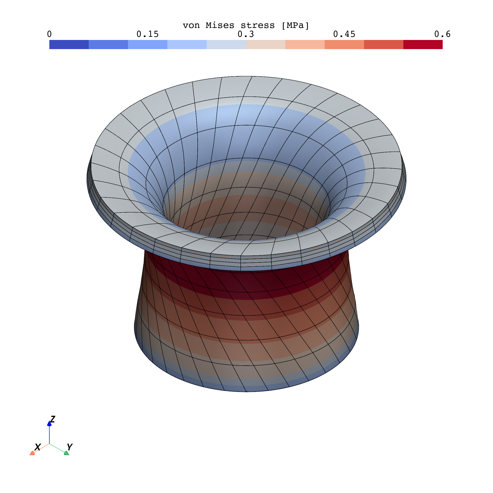
Source
plot_tube3d_pyvista(uo, so)Figure 2:Deformed tube coloured by von Mises stress at full torsional load.
- Pence, T. J., & Gou, K. (2014). On compressible versions of the incompressible neo-Hookean material. Mathematics and Mechanics of Solids, 20(2), 157–182. 10.1177/1081286514544258
- Habera, M., & Zilian, A. (2021). Symbolic spectral decomposition of 3x3 matrices. arXiv. 10.48550/ARXIV.2111.02117