Running error analysis for the Neo-Hookean strain energy density

This demo solves a Saint-Venant Kirchhoff problem for a 2D cantilever beam and computes the Neo-Hookean strain energy density. It demonstrates how to use running error analysis to obtain upper bounds or estimates on the running error accumulated during assembly.

In particular, this demo emphasizes:

custom assemblers that track rounding errors,
worst and exact error modes,
catastrophic cancellation in the standard Neo-Hookean energy density at small strains,
reformulation of the Neo-Hookean energy in terms of 3rd order expansion.

Background: Running error analysis¶

Running error analysis is an a posteriori method to estimate the numerical error in floating-point computations, see Chapter 3.3 of Higham (2002). Consider a floating-point operation on two inputs $\hat a$ and $\hat b$ that are already affected by some error from previous operations. The result $\hat y = \text{fl}(\hat a \text{ op } \hat b)$ satisfies

|\hat y - y^*| \leq \varepsilon |\hat y|,

(1)

where $\varepsilon$ is the machine epsilon (e.g. $\varepsilon = 2^{-52} \approx 2.22 \times 10^{-16}$ for double precision) and $y^* = \hat a \text{ op } \hat b$ is the exact result using the perturbed inputs. Both inputs carry errors $|\hat a - a| \leq \delta_a$ and $|\hat b - b| \leq \delta_b$ from previous operations. We can denote the exact result for unperturbed inputs as $y = a \text{ op } b$ . Then the total error $|\hat y - y|$ decomposes via the triangle inequality into two contributions:

|\hat y - y| \leq \underbrace{|\hat y - y^*|}_{\text{new rounding error}} + \underbrace{|y^* - y|}_{\text{propagated error}}.

(2)

Using first-order error analysis, i.e. expanding

y^* = y + \frac{\partial y}{\partial a} \delta_a + \frac{\partial y}{\partial b} \delta_b + \mathcal O(\delta_a^2, \delta_b^2, \delta_a \delta_b),

(3)

the propagated part is estimated as

|y^* - y| \leq \left|\frac{\partial y}{\partial a}\right| \delta_a + \left|\frac{\partial y}{\partial b}\right| \delta_b,

(4)

giving the combined running error bound

|\hat y - y| \leq \varepsilon |\hat y| + \left|\frac{\partial y}{\partial a}\right| \delta_a + \left|\frac{\partial y}{\partial b}\right| \delta_b.

(5)

The key insight is that this analysis can be carried out automatically alongside the computation by pairing each value with its error bound, which is exactly what the running_error_t<T> type in dolfiny implements. Each arithmetic operation updates both the value and the error bound according to the rules above, providing an approximate worst-case error bound at the end of the computation. This corresponds to ErrorMode::WORST, described in detail in the section on running error modes below.

This technique is known as running error analysis (or on-the-fly running error analysis): error bounds are propagated incrementally through every operation as the computation proceeds, rather than being derived symbolically beforehand or verified after the fact. It is cheap, requiring only one extra floating-point scalar per operation, and requires no change to the algorithm structure.

Running error modes: “worst” vs “exact”¶

The running_error_t<T> type supports two error-tracking strategies, selected at compile time via the ErrorMode template parameter.

ErrorMode::WORST (default). Each value is paired with a non-negative absolute error bound err_bnd. At every operation the bound is updated using the triangle inequality and first-order derivative propagation:

|\hat y - y| \leq \left|\frac{\partial y}{\partial a}\right| \delta_a + \left|\frac{\partial y}{\partial b}\right| \delta_b + \varepsilon |\hat{y}|.

(6)

Because absolute values of the derivatives are used throughout, errors can only accumulate and the bound can never decrease. This gives a rigorous, though potentially pessimistic, upper bound on the absolute error.

Note that the local rounding term uses the machine epsilon $\varepsilon = 2^{-52}$ rather than the unit roundoff $u = 2^{-53} = \varepsilon/2$ of round-to-nearest, so the per-operation contribution is a factor $\sim 2$ larger than strictly necessary. This is deliberate: it keeps the WORST bound a guaranteed (conservative) upper bound.

ErrorMode::EXACT. Each value is paired with a signed scalar exact_error that tracks the first-order propagated error with sign. The local rounding contribution at each step is computed exactly using MPFR arithmetic at 256-bit precision as the difference between the MPFR result and the native T result:

\hat y - y \approx \frac{\partial y}{\partial a} \, \delta_a + \frac{\partial y}{\partial b} \, \delta_b + \bigl(\hat{y} - y_{\mathrm{MPFR}}\bigr).

(7)

Because errors carry sign, contributions of opposite sign cancel, which reveals true cancellation in the computation rather than masking it under a worst-case envelope. This mode is more expensive (one MPFR call per scalar operation) but produces a tighter, signed estimate of the accumulated error.

C++ implementation: `running_error_t<T>`¶

The core of the running error analysis is a C++ struct running_error_t<T, Mode> (defined in running_error.h). The ErrorMode template parameter selects between the two tracking strategies. The WORST mode specialisation (default) pairs every floating-point value with a non-negative absolute error bound err_bnd:

template <typename T, ErrorMode Mode = ErrorMode::WORST>
struct running_error_t {
  using value_type = T;
  using re_t = running_error_t;
  T val;      // the computed value
  T err_bnd;  // accumulated absolute error bound (≥ 0)

  constexpr running_error_t(T _val = T(0), T _err = T(0)) noexcept
      : val(_val), err_bnd(_err) {}
  // ...
 private:
  static constexpr T eps = std::numeric_limits<T>::epsilon();
};

The EXACT mode specialisation replaces err_bnd with a signed exact_error field and adds a local_rounding helper that calls MPFR to compute the exact rounding contribution at each operation.

Every arithmetic operator is overloaded to update the error field alongside val. For WORST mode addition:

re_t operator+(const re_t& other) const {
  const T new_val = val + other.val;
  return re_t{new_val, err_bnd + other.err_bnd + eps * std::abs(new_val)};
}

Negation $y = -a$ is exact in IEEE 754 (sign bit flip, no rounding). In WORST mode the bound is simply inherited; in EXACT mode the signed error is negated:

// WORST mode
re_t operator-() const { return re_t{-val, err_bnd}; }

// EXACT mode
re_t operator-() const { return re_t{-val, -exact_error}; }

Non-linear functions abs, sqrt, log, and pow are overloaded in both modes with their analytic derivatives. In EXACT mode they additionally call MPFR to obtain the precise local rounding term. The struct also provides std::real, std::imag, and std::norm overloads so that FFCx’s templated assembly kernels, which may call these functions on the scalar type, compile and work correctly with running_error_t as a drop-in scalar type.

Python interface¶

On the Python side, running_error_t<double> has the same memory layout as std::complex<double> (two contiguous doubles), so the (val, err_bnd) pair maps directly onto complex128 with real = value and imag = error bound. This somewhat hacky reinterpretation is a necessary workaround because nanobind and DLPack only support a fixed set of scalar types (float32, float64, complex64, complex128, …) for zero-copy array exchange between C++ and Python. Custom structs like running_error_t cannot be described by DLPack’s dtype system. Since running_error_t<double> is layout-compatible with std::complex<double>, we simply expose the underlying buffer as complex128 without any copy or conversion. This means:

Input: coefficients are passed as complex128 arrays where real = value and imag = initial error. In this demo the input coefficients are treated as exact, so the error part is seeded with zero (imag = 0) and only the rounding accumulated during assembly is tracked. A representation-error seed such as $\varepsilon |v|$ could be supplied instead to also account for the inexactness of the inputs themselves.
Output: the assembled vector is a complex128 array where real = assembled value and imag = accumulated error after all assembly operations — an absolute upper bound in WORST mode, or a signed first-order estimate in EXACT mode.

The dolfiny.fem.form function JIT-compiles the UFL form using the running_error_t scalar type. To support this, we use the ffcx-backends library which provides templated kernels from FFCx, and we JIT compile these using cppyy. Finally, dolfiny.fem.assemble_vector invokes the DOLFINx assembly with this custom type, so every operation in the element kernel automatically tracks its error.

We start by generating a rectangular mesh for a cantilever beam.

from mpi4py import MPI
from petsc4py import PETSc

import basix
import dolfinx
import dolfinx.fem.petsc
import ufl

import gmsh
import numpy as np
import pyvista as pv

import dolfiny

comm = MPI.COMM_WORLD

w, h = 3.0, 0.8  # 3m long, 80cm high beam
res = 30

if comm.rank == 0:
    gmsh.initialize()
    gmsh.model.add("cantilever")
    gmsh.model.occ.addRectangle(0, 0, 0, w, h)
    gmsh.model.occ.synchronize()

    # Add physical groups for domain and boundaries
    gmsh.model.addPhysicalGroup(2, [1], name="domain")

    # Find left and right boundaries
    lines = gmsh.model.getEntities(1)
    left_line = None
    right_line = None
    for dim, tag in lines:
        com = gmsh.model.occ.getCenterOfMass(dim, tag)
        if np.isclose(com[0], 0.0):
            left_line = tag
        elif np.isclose(com[0], w):
            right_line = tag

    gmsh.model.addPhysicalGroup(1, [left_line], name="left")
    gmsh.model.addPhysicalGroup(1, [right_line], name="right")

    gmsh.option.setNumber("Mesh.MeshSizeMax", h / res)
    gmsh.model.mesh.generate(2)

mesh_data = dolfinx.io.gmsh.model_to_mesh(
    gmsh.model if comm.rank == 0 else None, comm, rank=0, gdim=2
)
mesh = mesh_data.mesh
fdim = mesh.topology.dim - 1
facet_tags = mesh_data.facet_tags
assert facet_tags is not None
tag_left = mesh_data.physical_groups["left"].tag
tag_right = mesh_data.physical_groups["right"].tag

if comm.rank == 0:
    gmsh.finalize()
    print("Number of cells:", mesh.topology.index_map(mesh.topology.dim).size_local)

Info    : Meshing 1D...
Info    : [  0%] Meshing curve 1 (Line)
Info    : [ 30%] Meshing curve 2 (Line)
Info    : [ 60%] Meshing curve 3 (Line)
Info    : [ 80%] Meshing curve 4 (Line)
Info    : Done meshing 1D (Wall 0.000510544s, CPU 0.000806s)
Info    : Meshing 2D...
Info    : Meshing surface 1 (Plane, Frontal-Delaunay)
Info    : Done meshing 2D (Wall 0.135225s, CPU 0.135606s)
Info    : 4105 nodes 8212 elements
Number of cells: 7922

Linear elasticity¶

We solve a standard linear elasticity problem with steel-like properties. The beam is clamped on the left boundary and subjected to a downward traction on the right boundary.

Ve = basix.ufl.element("P", mesh.basix_cell(), 1, shape=(mesh.geometry.dim,))
V = dolfinx.fem.functionspace(mesh, Ve)

u0_svk = dolfinx.fem.Function(V, name="displacement_svk")

# Steel properties
E = 200e9  # 200 GPa
nu = 0.3
mu = E / (2.0 * (1.0 + nu))

# Plane strain
lmbda = E * nu / ((1.0 + nu) * (1.0 - 2.0 * nu))
kappa = E / (3.0 * (1.0 - 2.0 * nu))


def GL(u):
    return 0.5 * (ufl.grad(u) + ufl.grad(u).T + ufl.grad(u).T * ufl.grad(u))


ds = ufl.Measure("ds", domain=mesh, subdomain_data=facet_tags)

# Traction load on the right boundary
f = np.array([0.0, -10e2], dtype=np.float64)
T = dolfinx.fem.Constant(mesh, f)

energy_load = ufl.inner(T, u0_svk) * ds(tag_right)
energy_svk = (
    lmbda / 2 * ufl.tr(GL(u0_svk)) ** 2 * ufl.dx
    + mu * ufl.inner(GL(u0_svk), GL(u0_svk)) * ufl.dx
    - energy_load
)

F_svk = ufl.derivative(energy_svk, u0_svk)

left_dofs = dolfinx.fem.locate_dofs_topological(V, fdim, facet_tags.find(tag_left))
bc = dolfinx.fem.dirichletbc(np.zeros(mesh.geometry.dim, dtype=np.float64), left_dofs, V)

opts = PETSc.Options("svk")  # type: ignore[attr-defined]
opts["ksp_type"] = "preonly"
opts["pc_type"] = "lu"
opts["pc_factor_mat_solver_type"] = "mumps"

problem = dolfiny.snesproblem.SNESProblem([F_svk], [u0_svk], bcs=[bc], prefix="svk")

_ = problem.solve()

# SNES iteration  0

# sub  0 [  8k] |x|=0.000e+00 |dx|=0.000e+00 |r|=1.448e+02 (displacement_svk)

# all           |x|=0.000e+00 |dx|=0.000e+00 |r|=1.448e+02

# SNES iteration  0, KSP iteration   0       |r|=1.448e+02

# SNES iteration  0, KSP iteration   1       |r|=3.185e-09

# SNES iteration  1

# sub  0 [  8k] |x|=2.569e-05 |dx|=2.569e-05 |r|=8.826e-03 (displacement_svk)

# all           |x|=2.569e-05 |dx|=2.569e-05 |r|=8.826e-03

# SNES iteration  1, KSP iteration   0       |r|=8.826e-03

# SNES iteration  1, KSP iteration   1       |r|=4.797e-16

# SNES iteration  2 success = CONVERGED_FNORM_RELATIVE

# sub  0 [  8k] |x|=2.569e-05 |dx|=3.765e-12 |r|=7.894e-10 (displacement_svk)

# all           |x|=2.569e-05 |dx|=3.765e-12 |r|=7.894e-10

Neo-Hookean strain energy density with running error bounds¶

To track running errors through the strain energy computation, we assemble two forms of the strain energy density using the running error bound implementation and compare their running error behaviour.

Full Neo-Hookean (numerically unstable). The standard Neo-Hookean strain energy density in 2D reads

W = \frac{\mu}{2}(I_1 - 2 - 2\ln J) + \frac{\kappa}{2}(J-1)^2,

(8)

where $I_1 = \text{Tr}(\mathbf{C})$ , $J = \det(\mathbf{F})$ , $\mathbf{C} = \mathbf{F}^T \mathbf{F}$ , and $\mathbf{F} = \mathbf{I} + \nabla\mathbf{u}$ , is known to be numerically unstable for small deformations, see Shakeri et al. (2024). The instability comes from catastrophic cancellation in $I_1 - 2 - 2\ln J$ when $I_1 \approx 2$ and $J \approx 1$ (small strains), and similarly in $(J-1)^2$ when $J \approx 1$ .

Second- and third-order expansion in the Green-Lagrange strain. Following Habera & Zilian (2026), the cancellation can be avoided by reformulating the energy in terms of the Green-Lagrange strain $\mathbf{E} = \tfrac{1}{2}(\mathbf{C} - \mathbf{I})$ , which acts on the displacement gradient $\mathbf{H} = \nabla\mathbf{u}$ directly so that the identity term in $\mathbf{F}$ is eliminated. Splitting $\mathbf{E}$ into a linear and a nonlinear part,

\mathbf{E} = \mathbf{E}_1 + \mathbf{E}_2, \qquad \mathbf{E}_1 = \tfrac{1}{2}\bigl(\nabla\mathbf{u} + \nabla\mathbf{u}^\mathsf{T}\bigr), \qquad \mathbf{E}_2 = \tfrac{1}{2}\,\nabla\mathbf{u}^\mathsf{T}\nabla\mathbf{u},

(9)

the two contributions scale as $\mathbf{E}_1 = \mathcal{O}(\Pi_3)$ and $\mathbf{E}_2 = \mathcal{O}(\Pi_3^2)$ , where $\Pi_3 = u_\mathrm{ref}/l_\mathrm{ref}$ is the dimensionless deformation group identified in the dimensional analysis. With $I_1 = \operatorname{tr}(\mathbf{I} + 2\mathbf{E})$ and $J = \sqrt{\det(\mathbf{I} + 2\mathbf{E})}$ , the isochoric part reduces to $\mu\,(\operatorname{tr}\mathbf{E} - \ln J)$ . Expanding both parts to third order in $\Pi_3$ gives $\tilde W = \tilde W^{(2)} + \tilde W^{(3)} + \mathcal{O}(\Pi_3^4)$ with

\begin{aligned} \tilde W^{(2)} &= \underbrace{\mu\,\operatorname{tr}(\mathbf{E}_1^2)}_{\tilde W^{(2)}_\mu} + \underbrace{\tfrac{\kappa}{2}\,\operatorname{tr}(\mathbf{E}_1)^2}_{\tilde W^{(2)}_\kappa}, \\ \tilde W^{(3)} &= \underbrace{\mu\bigl(2\,\mathbf{E}_1 : \mathbf{E}_2 - \tfrac{4}{3}\operatorname{tr}(\mathbf{E}_1^3)\bigr)}_{\tilde W^{(3)}_\mu} + \underbrace{\kappa\bigl(\operatorname{tr}(\mathbf{E}_1)\operatorname{tr}(\mathbf{E}_2) + \tfrac{1}{2}\operatorname{tr}(\mathbf{E}_1)^3 - \operatorname{tr}(\mathbf{E}_1)\operatorname{tr} (\mathbf{E}_1^2)\bigr)}_{\tilde W^{(3)}_\kappa}. \end{aligned}

(10)

These are the four terms shear_2, bulk_2, shear_3, bulk_3 of Habera & Zilian (2026), each homogeneous in the dimensional quantities $\mu$ , $\kappa$ , $l_\mathrm{ref}$ , and $u_\mathrm{ref}$ . The volumetric terms use the bulk modulus $\kappa$ (consistent with the $\tfrac{\kappa}{2}(J-1)^2$ term of the full energy above), and the expansion is expected to carry a much smaller relative running error at small strains than the unstable $I_1 - 2 - 2\ln J$ and $(J-1)^2$ form.

Both forms are assembled with the running error bound implementation. The output is a complex128 vector: the real part is the assembled strain energy density value and the imaginary part is the accumulated absolute error bound. The two forms are compared side-by-side in the visualisation below.

Assembling strain energy with running error bounds¶

We define a helper function extract_energy_fields that compiles UFL forms using the running error implementation, assembles them with automatic error tracking, and extracts the computed values alongside their accumulated error bounds.

The assembly process works as follows:

Compile the form using dolfiny.fem.form() with the running error type
Assemble the vector using dolfiny.fem.assemble_vector(), which tracks errors throughout all element kernel operations
Extract results from the complex-valued output where real = value and imag = accumulated error bound
Compare timing against standard DOLFINx assembly to measure the computational overhead

The function supports both "worst" (pessimistic but rigorous) and "exact" (tighter, signed) error modes.

# DG-0 space for cell-wise strain energy density
S = dolfinx.fem.functionspace(mesh, ("DG", 0))
δs = ufl.TestFunction(S)


def extract_energy_fields(form, name, suffix="", mode="worst"):
    """Compile form, assemble vector, and extract values and error bounds."""
    import time

    compiled_form = dolfiny.fem.form(form, mode=mode)
    t0 = time.time()
    b = dolfiny.fem.assemble_vector(compiled_form)
    time_dolfiny = time.time() - t0

    compiled_form_dolfinx = dolfinx.fem.form(form)
    t0 = time.time()
    _ = dolfinx.fem.petsc.assemble_vector(compiled_form_dolfinx)
    time_dolfinx = time.time() - t0

    slowdown = time_dolfiny / time_dolfinx if time_dolfinx > 0 else float("inf")
    if comm.rank == 0:
        print(f"{name:41s} ({mode:5s} mode): {time_dolfiny:8.2g}s (slowdown: {slowdown:6.2f}x)")

    energy = dolfinx.fem.Function(S, name=name)
    energy.x.array[:] = b.real

    abs_err = dolfinx.fem.Function(S, name=f"absolute_error{suffix}_{mode}")
    abs_err.x.array[:] = np.abs(b.imag)

    rel_err = dolfinx.fem.Function(S, name=f"relative_error{suffix}_{mode}")
    nonzero = np.abs(b.real) > 0
    rel_err.x.array[nonzero] = abs_err.x.array[nonzero] / np.abs(b.real[nonzero])

    return energy, abs_err, rel_err


# --- 1) Neo-Hookean strain energy density ---
dim = mesh.geometry.dim
F = ufl.Identity(dim) + ufl.grad(u0_svk)
C = F.T * F
I1, J = ufl.tr(C), ufl.det(F)

energy = mu / 2 * (I1 - 2 - 2 * ufl.ln(J)) + kappa / 2 * (J - 1) ** 2
energy_form = (energy / ufl.CellVolume(mesh)) * δs * ufl.dx

energy_fn, abs_error_fn, rel_error_fn = extract_energy_fields(energy_form, "Strain Energy Density")
energy_fn_exact, abs_error_fn_exact, rel_error_fn_exact = extract_energy_fields(
    energy_form, "Strain Energy Density", mode="exact"
)

H = ufl.grad(u0_svk)
E1 = ufl.sym(H)
E2 = 0.5 * H.T * H

# Second-order terms
shear_2 = mu * ufl.tr(E1 * E1)  # W^(2)_mu
bulk_2 = kappa / 2 * ufl.tr(E1) ** 2  # W^(2)_kappa

# Third-order terms
shear_3 = mu * (2 * ufl.inner(E1, E2) - 4 / 3 * ufl.tr(E1 * E1 * E1))  # W^(3)_mu
bulk_3 = kappa * (
    ufl.tr(E1) * ufl.tr(E2) + 1 / 2 * ufl.tr(E1) ** 3 - ufl.tr(E1) * ufl.tr(E1 * E1)
)  # W^(3)_kappa

energy_approx = shear_2 + bulk_2 + shear_3 + bulk_3
energy_approx_form = (energy_approx / ufl.CellVolume(mesh)) * δs * ufl.dx

energy_approx_fn, abs_error_approx_fn, rel_error_approx_fn = extract_energy_fields(
    energy_approx_form, "Neo-Hooke Expansion Strain Energy Density", suffix="_approx"
)
energy_approx_fn_exact, abs_error_approx_fn_exact, rel_error_approx_fn_exact = (
    extract_energy_fields(
        energy_approx_form,
        "Neo-Hooke Expansion Strain Energy Density",
        suffix="_approx",
        mode="exact",
    )
)

# Write results
with dolfinx.io.XDMFFile(comm, "error.xdmf", "w") as xdmf:
    xdmf.write_mesh(mesh)
    xdmf.write_function(u0_svk)
    xdmf.write_function(energy_fn)
    xdmf.write_function(rel_error_fn)
    xdmf.write_function(abs_error_fn)
    xdmf.write_function(rel_error_fn_exact)

Strain Energy Density                     (worst mode):   0.0012s (slowdown:   1.37x)

Strain Energy Density                     (exact mode):     0.21s (slowdown: 233.70x)

Neo-Hooke Expansion Strain Energy Density (worst mode):   0.0019s (slowdown:   2.01x)

Neo-Hooke Expansion Strain Energy Density (exact mode):     0.22s (slowdown: 223.37x)

Visualisation¶

def frame_beam(plotter):
    """Frame the beam tightly, leaving headroom for the horizontal colorbar."""
    plotter.view_xy()
    plotter.camera.zoom(2.9)
    # Shift the view upwards so the beam sits below the colorbar.
    fx, fy, fz = plotter.camera.focal_point
    px, py, pz = plotter.camera.position
    plotter.camera.focal_point = (fx, fy + 0.1 * h, fz)
    plotter.camera.position = (px, py + 0.1 * h, pz)


if comm.size == 1:
    # Create pyvista grid
    grid = pv.UnstructuredGrid(*dolfinx.plot.vtk_mesh(mesh))

    # Add data to grid
    grid.cell_data["Neo-Hooke Unstable [Pa]"] = energy_fn.x.array
    grid.cell_data["Rel. Error Bound (unstable, WORST) [-]"] = np.abs(rel_error_fn.x.array)
    grid.cell_data["Neo-Hooke 3rd Order Expansion [Pa]"] = energy_approx_fn.x.array
    grid.cell_data["Rel. Error Bound (expansion, WORST) [-]"] = np.abs(rel_error_approx_fn.x.array)
    grid.cell_data["Rel. Error Bound (unstable, EXACT) [-]"] = np.abs(rel_error_fn_exact.x.array)
    grid.cell_data["Rel. Error Bound (expansion, EXACT) [-]"] = np.abs(
        rel_error_approx_fn_exact.x.array
    )

    n_colors = 30
    show_edges = False
    energy_clim = (
        energy_approx_fn.x.array.min(),
        energy_approx_fn.x.array.max(),
    )

    window_width = dolfiny.pyvista.pixels
    window_height = dolfiny.pyvista.pixels // 3
    dolfiny.pyvista.theme.colorbar_horizontal.position_y = 0.83

    # --- Plot 1: Neo-Hooke unstable energy ---
    plotter1 = pv.Plotter(
        off_screen=True,
        theme=dolfiny.pyvista.theme,
        window_size=(window_width, window_height),
        border=False,
    )
    plotter1.add_mesh(
        grid.copy(deep=False),
        scalars="Neo-Hooke Unstable [Pa]",
        n_colors=n_colors,
        log_scale=True,
        clim=energy_clim,
        show_edges=show_edges,
    )
    frame_beam(plotter1)

    plotter1.screenshot("energy_unstable.png")
    plotter1.close()
    plotter1.deep_clean()

    # --- Plot 2: Neo-Hooke 3rd order expansion energy ---
    plotter2 = pv.Plotter(
        off_screen=True,
        theme=dolfiny.pyvista.theme,
        window_size=(window_width, window_height),
        border=False,
    )
    plotter2.add_mesh(
        grid.copy(deep=False),
        scalars="Neo-Hooke 3rd Order Expansion [Pa]",
        n_colors=n_colors,
        log_scale=True,
        clim=energy_clim,
        show_edges=show_edges,
    )
    frame_beam(plotter2)

    plotter2.screenshot("energy_expansion.png")
    plotter2.close()
    plotter2.deep_clean()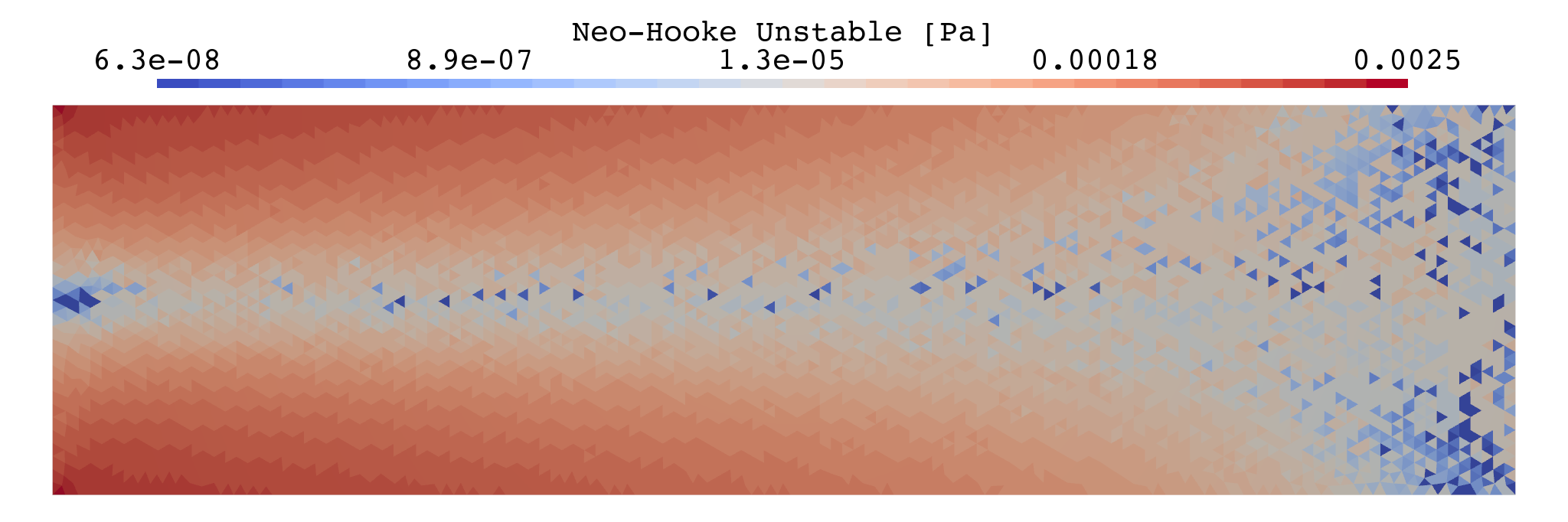

(a)Neo-Hookean strain energy density, unstable formulation.

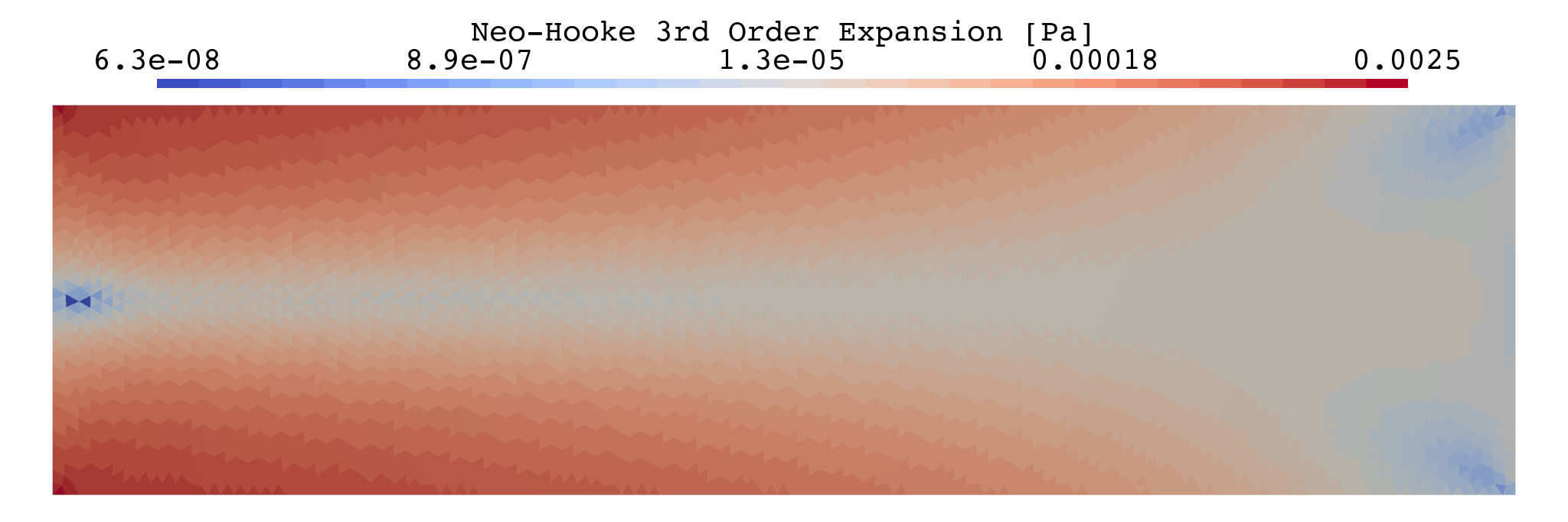
Neo-Hookean strain energy density, 3rd-order expansion. — (a)Neo-Hookean strain energy density, unstable formulation.

if comm.size == 1:
    # Create pyvista grid
    grid = pv.UnstructuredGrid(*dolfinx.plot.vtk_mesh(mesh))

    # Add data to grid
    grid.cell_data["Rel. Error Bound (unstable, WORST) [-]"] = np.abs(rel_error_fn.x.array)
    grid.cell_data["Rel. Error Bound (unstable, EXACT) [-]"] = np.abs(rel_error_fn_exact.x.array)

    show_edges = False

    window_width = dolfiny.pyvista.pixels
    window_height = dolfiny.pyvista.pixels // 3
    dolfiny.pyvista.theme.colorbar_horizontal.position_y = 0.83

    # --- Plot 3: Unstable error, WORST mode ---
    plotter3 = pv.Plotter(
        off_screen=True,
        theme=dolfiny.pyvista.theme,
        window_size=(window_width, window_height),
        border=False,
    )
    plotter3.add_mesh(
        grid.copy(deep=False),
        scalars="Rel. Error Bound (unstable, WORST) [-]",
        log_scale=True,
        n_colors=n_colors,
        show_edges=show_edges,
    )
    frame_beam(plotter3)

    plotter3.screenshot("error_unstable_worst.png")
    plotter3.close()
    plotter3.deep_clean()

    # --- Plot 4: Unstable error, EXACT mode ---
    plotter4 = pv.Plotter(
        off_screen=True,
        theme=dolfiny.pyvista.theme,
        window_size=(window_width, window_height),
        border=False,
    )
    plotter4.add_mesh(
        grid.copy(deep=False),
        scalars="Rel. Error Bound (unstable, EXACT) [-]",
        log_scale=True,
        n_colors=n_colors,
        show_edges=show_edges,
    )
    frame_beam(plotter4)

    plotter4.screenshot("error_unstable_exact.png")
    plotter4.close()
    plotter4.deep_clean()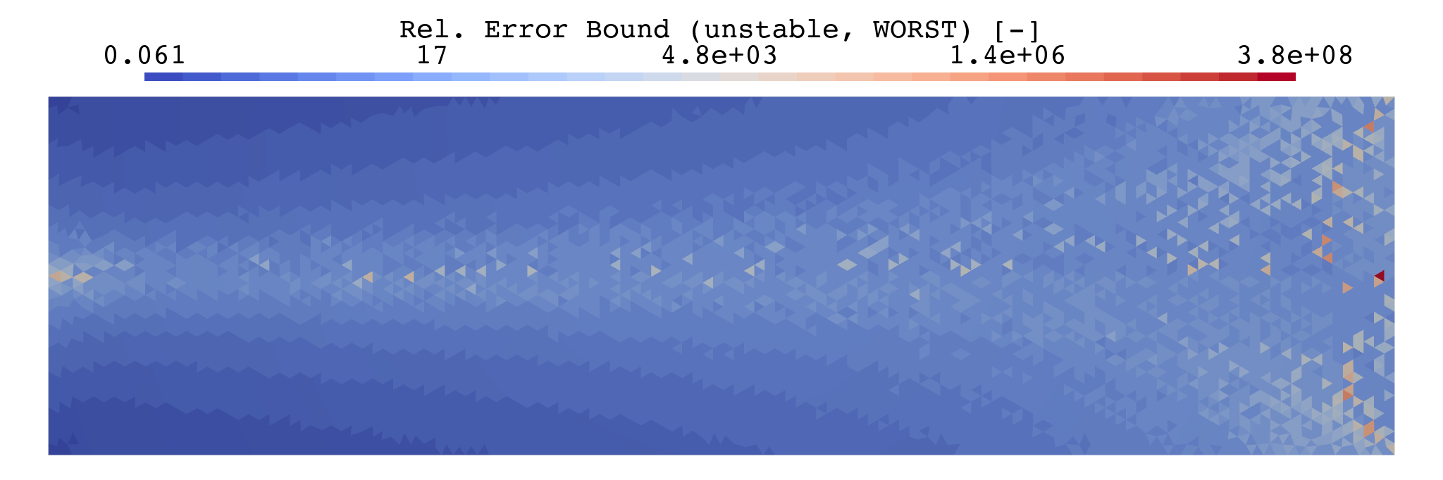

(a)Running error bound, unstable formulation, WORST mode.

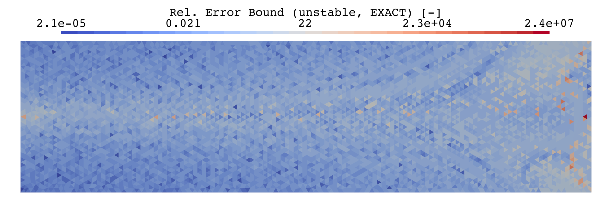
Running error estimate, unstable formulation, EXACT mode. — (a)Running error bound, unstable formulation, WORST mode.

if comm.size == 1:
    # Create pyvista grid
    grid = pv.UnstructuredGrid(*dolfinx.plot.vtk_mesh(mesh))

    # Add data to grid
    grid.cell_data["Rel. Error Bound (expansion, WORST) [-]"] = np.abs(rel_error_approx_fn.x.array)
    grid.cell_data["Rel. Error Bound (expansion, EXACT) [-]"] = np.abs(
        rel_error_approx_fn_exact.x.array
    )

    show_edges = False

    window_width = dolfiny.pyvista.pixels
    window_height = dolfiny.pyvista.pixels // 3
    dolfiny.pyvista.theme.colorbar_horizontal.position_y = 0.83

    # --- Plot 5: Expansion error, WORST mode ---
    plotter5 = pv.Plotter(
        off_screen=True,
        theme=dolfiny.pyvista.theme,
        window_size=(window_width, window_height),
        border=False,
    )
    plotter5.add_mesh(
        grid.copy(deep=False),
        scalars="Rel. Error Bound (expansion, WORST) [-]",
        log_scale=True,
        n_colors=n_colors,
        show_edges=show_edges,
    )
    frame_beam(plotter5)

    plotter5.screenshot("error_expansion_worst.png")
    plotter5.close()
    plotter5.deep_clean()

    # --- Plot 6: Expansion error, EXACT mode ---
    plotter6 = pv.Plotter(
        off_screen=True,
        theme=dolfiny.pyvista.theme,
        window_size=(window_width, window_height),
        border=False,
    )
    plotter6.add_mesh(
        grid.copy(deep=False),
        scalars="Rel. Error Bound (expansion, EXACT) [-]",
        log_scale=True,
        n_colors=n_colors,
        show_edges=show_edges,
    )
    frame_beam(plotter6)

    plotter6.screenshot("error_expansion_exact.png")
    plotter6.close()
    plotter6.deep_clean()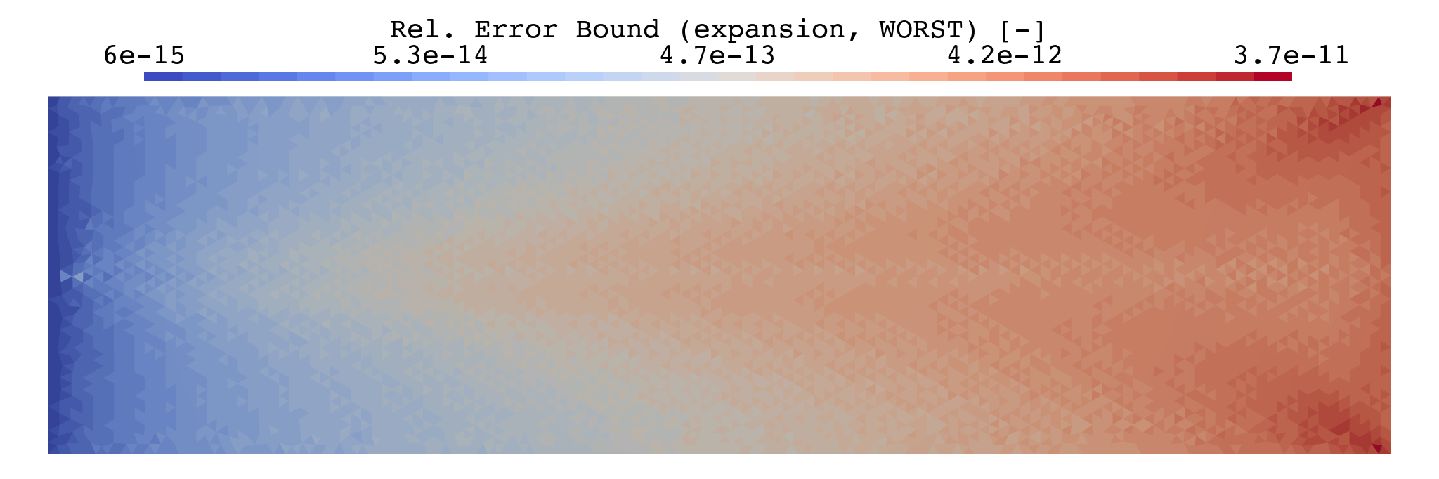

(a)Running error bound, 3rd-order expansion, WORST mode.

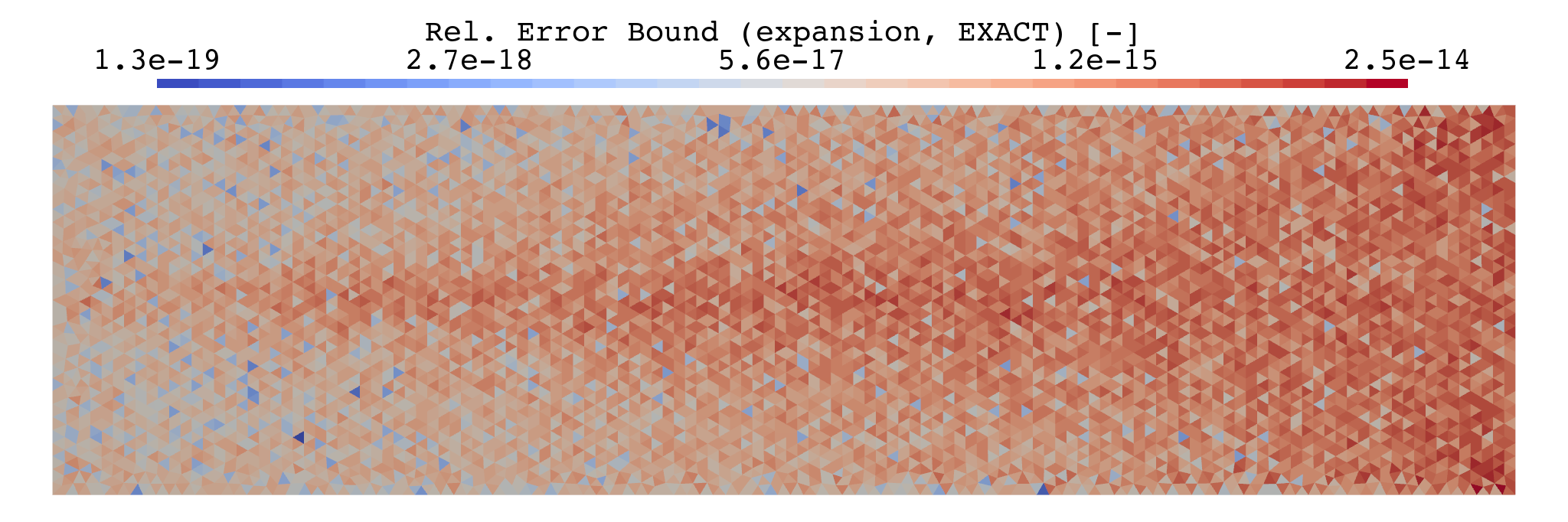
Running error estimate, 3rd-order expansion, EXACT mode. — (a)Running error bound, 3rd-order expansion, WORST mode.