This demo demonstrates the automated dimensional analysis in dolfiny.units on a transient
incompressible Navier-Stokes lid-driven cavity problem. The demo does not solve the nonlinear
cavity problem. Instead, it assembles the Jacobian of the normalized residual at the zero state
and studies how its matrix condition number varies with the Euler number.
We start from dimensional reference quantities, check the weak form, and normalize the residual by the convective scale. The resulting Reynolds, Euler, Froude, and Strouhal dimensionless numbers emerge directly from the UFL form.
In particular this demo emphasises
automated Buckingham Pi analysis and dimensional checks for a UFL model,
extraction of Reynolds, Euler, Froude, and Strouhal numbers by normalising the weak form, and
how the conditioning of the normalised Navier-Stokes Jacobian changes under pressure scaling.
Model
On the unit square we consider velocity and pressure such that the incompressible Navier-Stokes equations in the strong form read
Here is the spatial domain, denotes the time derivative, denotes the spatial gradient or divergence as appropriate, and is the identity tensor. Furthermore, is the strain-rate tensor, is the density, is the kinematic viscosity, is a gravity scale, and is a dimensionless body-force direction.
Source
import argparse
import sys

from mpi4py import MPI

import basix
import dolfinx
import dolfinx.fem.petsc
import ufl
from dolfinx import default_scalar_type as scalar

import matplotlib.pyplot as plt
import numpy as np
import sympy.physics.units as syu

import dolfiny
import dolfiny.la
from dolfiny.units import Quantity

default_p_ref = 5000.0


def get_args(argv=None):
    parser = argparse.ArgumentParser(description="Navier-Stokes dimensional analysis")
    parser.add_argument(
        "--p-ref-min",
        type=float,
        default=100.0,
        help="Minimum reference pressure value in the sweep (default: 100.0)",
    )
    parser.add_argument(
        "--p-ref-max",
        type=float,
        default=10000.0,
        help="Maximum reference pressure value in the sweep (default: 10000.0)",
    )
    parser.add_argument(
        "--num-p-ref",
        type=int,
        default=20,
        help="Number of reference pressure values in the sweep (default: 20)",
    )
    parser.add_argument(
        "--plot-file",
        default="navier_stokes_condition_number.png",
        help="Filename of the condition-number plot (default: navier_stokes_condition_number.png)",
    )

    if argv is None and "ipykernel" in sys.modules:
        argv = []  # ignore Jupyter's own args

    return parser.parse_args(argv)


args = get_args()
comm = MPI.COMM_WORLD

if comm.size != 1:
    raise RuntimeError(
        "This demo computes dense condition numbers with NumPy and must be run with one MPI rank."
    )

mesh = dolfinx.mesh.create_unit_square(comm, 10, 10)
Ve = basix.ufl.element("P", mesh.basix_cell(), 2, shape=(mesh.topology.dim,))
Pe = basix.ufl.element("P", mesh.basix_cell(), 1)
Vf = dolfinx.fem.functionspace(mesh, Ve)
Pf = dolfinx.fem.functionspace(mesh, Pe)

v = dolfinx.fem.Function(Vf, name="v")
v0 = dolfinx.fem.Function(Vf, name="v0")  # velocity at the previous time level
p = dolfinx.fem.Function(Pf, name="p")
δv, δp = ufl.TestFunctions(ufl.MixedFunctionSpace(Vf, Pf))  # velocity and pressure test functions

b = dolfinx.fem.Constant(mesh, (0.0, -1.0))  # dimensionless body-force direction
num_steps_per_t_ref = dolfinx.fem.Constant(mesh, scalar(1))  # dt = t_ref / num_steps_per_t_ref
Reference quantities and nondimensional groups
The dimensional model is described by the reference scales. The subscript ref marks prescribed
dimensional scales used to normalize the equations.
| Symbol | Value | Meaning |
|---|---|---|
| kinematic viscosity | ||
| density | ||
| reference length | ||
| reference time | ||
| reference velocity | ||
| representative value , then swept | reference pressure | |
| gravity scale |
Each scale is created as a Quantity(mesh, scale, unit, symbol). Quantity is a
dolfinx.fem.Constant with extra metadata: besides the scalar value used in assembly, it stores
the unit, SymPy-based symbol, and derived dimension used for Buckingham Pi analysis and
dimensional checks.
Buckingham Pi analysis below reports the basis (so-called Pi groups) of the nullspace of the dimension matrix. For this problem, there are four Pi groups:
A call to dolfiny.units.buckingham_pi_analysis with a list of Quantity objects
reports the overview of all dimensional quantities in the model, the dimension matrix, and the
Pi groups. Please note, that Pi groups are found using a Matrix.nullspace() call in SymPy.
For matrices over the field of rational numbers, the nullspace is usually represented
with small integer coefficients, which is favorable for interpretability.
Source
nu = Quantity(mesh, 1000, syu.millimeter**2 / syu.second, "nu")
rho = Quantity(mesh, 5000, syu.kilogram / syu.m**3, "rho")
l_ref = Quantity(mesh, 1, syu.meter, "l_ref")
t_ref = Quantity(mesh, 1 / 60, syu.minute, "t_ref")
v_ref = Quantity(mesh, 1, syu.meter / syu.second, "v_ref")
p_ref = Quantity(mesh, default_p_ref, syu.pascal, "p_ref")
g_ref = Quantity(mesh, 10, syu.meter / syu.second**2, "g_ref")
quantities = [v_ref, l_ref, rho, nu, g_ref, p_ref, t_ref]  # order -> Pi_1, ..., Pi_4

if comm.rank == 0:
    dolfiny.units.buckingham_pi_analysis(quantities)
==================================================
Buckingham Pi Analysis
==================================================
Symbol | Expression | Value (in base units)
-------+-----------------------------+----------------------------------
v_ref | meter/second | meter/second
l_ref | meter | meter
rho | 5000.0*kilogram/meter**3 | 5000.0*kilogram/meter**3
nu | 1000.0*millimeter**2/second | 0.001*meter**2/second
g_ref | 10.0*meter/second**2 | 10.0*meter/second**2
p_ref | 5000.0*pascal | 5000.0*kilogram/(meter*second**2)
t_ref | 0.01667*minute | 1.0*second
Dimension matrix (7 x 7):
Dimension | v_ref | l_ref | rho | nu | g_ref | p_ref | t_ref
--------------------+-------+-------+-----+----+-------+-------+------
amount_of_substance | 0 | 0 | 0 | 0 | 0 | 0 | 0
current | 0 | 0 | 0 | 0 | 0 | 0 | 0
length | 1 | 1 | -3 | 2 | 1 | -1 | 0
luminous_intensity | 0 | 0 | 0 | 0 | 0 | 0 | 0
mass | 0 | 0 | 1 | 0 | 0 | 1 | 0
temperature | 0 | 0 | 0 | 0 | 0 | 0 | 0
time | -1 | 0 | 0 | -1 | -2 | -2 | 1
Dimensionless groups (4):
Group | Expression | Value
------+----------------------+------
Pi_1 | nu/(l_ref*v_ref) | 0.001
Pi_2 | g_ref*l_ref/v_ref**2 | 10
Pi_3 | p_ref/(rho*v_ref**2) | 1
Pi_4 | t_ref*v_ref/l_ref | 1
==================================================
Weak form and dimensional checks
We write the residual in term-by-term form so that each contribution can be transformed and factorized independently. We want to find such that the residual for all test functions . Here denotes the velocity at the previous time level, and is the number of time steps per reference time so that :
with
Here denotes the Frobenius product of tensors and denotes integration over
.
The last term is identically zero. It is kept only so that DOLFINx allocates a pressure-pressure
sparsity block, allowing the pressure pinning condition to modify a diagonal entry there. The
factor is only a dimensional placeholder inside this zero
term.
The dictionary mapping below connects the dimensionless coordinates, unknowns, and test
functions to their dimensional counterparts: coordinates scale with , velocity
with , and pressure with .
The mapping applies the following transformations:
After the transformation, we proceed with the steps: factorization and normalization. Factorization performs a homogeneous factorization of the weak form and extracts the homogeneous factors. Normalization then divides each term by a chosen reference term, which is the convection term in this case. The resulting dimensionless form contains only the Pi groups as coefficients.
Source
mapping = {
    mesh.ufl_domain(): l_ref,
    v: v_ref * v,
    v0: v_ref * v0,
    p: p_ref * p,
    δv: v_ref * δv,
    δp: p_ref * δp,
}


def D(u_expr):
    """Strain rate tensor."""
    return ufl.sym(ufl.grad(u_expr))


terms = {
    "unsteady": ufl.inner(δv, rho * (v - v0) / (t_ref / num_steps_per_t_ref)) * ufl.dx,
    "convection": ufl.inner(δv, rho * ufl.dot(v, ufl.grad(v))) * ufl.dx,
    "viscous": ufl.inner(D(δv), 2 * rho * nu * D(v)) * ufl.dx,
    "pressure": -ufl.inner(ufl.div(δv), p) * ufl.dx,
    "force": -ufl.inner(δv, rho * g_ref * b) * ufl.dx,
    "incompressibility": δp * ufl.div(v) * ufl.dx,
    "pressure_bc": -dolfinx.fem.Constant(mesh, 0.0) / p_ref / t_ref * ufl.inner(δp, p) * ufl.dx,
}


# Few dimensional sanity checks
dimsys = syu.si.SI.get_dimension_system()
assert dimsys.equivalent_dims(dolfiny.units.get_dimension(D(v), quantities, mapping), 1 / syu.time)
assert dimsys.equivalent_dims(
    dolfiny.units.get_dimension(
        rho * (v - v0) / (t_ref / num_steps_per_t_ref), quantities, mapping
    ),
    syu.mass / syu.length**3 * syu.length / syu.time**2,
)
assert dolfiny.units.get_dimension(D(v), quantities, mapping) == 1 / syu.time

form = sum(terms.values(), ufl.form.Zero())
form_dim = dolfiny.units.get_dimension(form, quantities, mapping)
assert dimsys.equivalent_dims(form_dim, syu.power / syu.length)

convective_dim = dolfiny.units.get_dimension(rho * ufl.dot(v, ufl.grad(v)), quantities, mapping)
assert syu.si.SI.get_dimension_system().equivalent_dims(convective_dim, syu.force / syu.length**3)

terms_fact = dolfiny.units.factorize(terms, quantities, mode="factorize", mapping=mapping)
assert isinstance(terms_fact, dict)

reference_term = "convection"

terms_norm = dolfiny.units.normalize(terms_fact, reference_term, quantities)
==================================================
Terms after normalization with "convection"
==================================================
Reference factor from 'convection':
Term | Factor | Value (in base units)
-----------+--------------------+--------------------------------
convection | l_ref*rho*v_ref**3 | 5000.0*kilogram*meter/second**3
Term | Factor | Value (in base units)
------------------+----------------------------------+----------------------
unsteady | l_ref/(t_ref*v_ref) | 1.000
convection | 1 | 1.000
viscous | nu/(l_ref*v_ref) | 0.001000
pressure | p_ref/(rho*v_ref**2) | 1.000
force | g_ref*l_ref/v_ref**2 | 10.00
incompressibility | p_ref/(rho*v_ref**2) | 1.000
pressure_bc | l_ref*p_ref/(rho*t_ref*v_ref**3) | 1.000
==================================================
Source
form_nondimensional = sum(terms_norm.values(), ufl.form.Zero())Lid-driven cavity boundary conditions
The normalized residual uses standard lid-driven cavity boundary data: no-slip on the left, right, and bottom boundaries, unit tangential velocity on the lid, and one pressure degree of freedom fixed at the corner point to remove the constant nullspace. This keeps the conditioning study focused on the reference scaling rather than on an undetermined pressure level. The gravity term is retained only so that the dimensional analysis also exposes the corresponding Froude dimensionless number.
Source
def noslip_boundary(x):
    return np.isclose(x[0], 0.0) | np.isclose(x[0], 1.0) | np.isclose(x[1], 0.0)


def lid(x):
    return np.isclose(x[1], 1.0)


def lid_velocity_expression(x):
    return np.stack((np.ones(x.shape[1]), np.zeros(x.shape[1])))


noslip = np.zeros(mesh.geometry.dim, dtype=scalar)
facets = dolfinx.mesh.locate_entities_boundary(mesh, 1, noslip_boundary)
bc0 = dolfinx.fem.dirichletbc(noslip, dolfinx.fem.locate_dofs_topological(Vf, 1, facets), Vf)

lid_velocity = dolfinx.fem.Function(Vf)
lid_velocity.interpolate(lid_velocity_expression)
facets = dolfinx.mesh.locate_entities_boundary(mesh, 1, lid)
bc1 = dolfinx.fem.dirichletbc(lid_velocity, dolfinx.fem.locate_dofs_topological(Vf, 1, facets))

dof0 = dolfinx.fem.locate_dofs_geometrical(
    Pf, lambda x: np.isclose(x[0], 0.0) & np.isclose(x[1], 0.0)
)
bc2 = dolfinx.fem.dirichletbc(scalar(0.0), dof0, Pf)

bcs = [bc0, bc1, bc2]
Matrix conditioning under pressure scaling
We assemble the Jacobian matrix of the mixed residual at the zero state for a sequence of pressure scales. The Jacobian is assembled into a
PETSc MATAIJ matrix, converted to SciPy CSR format with dolfiny.la.petsc_to_scipy,
and then densified only for the call to numpy.linalg.cond, which estimates the spectral
condition number .
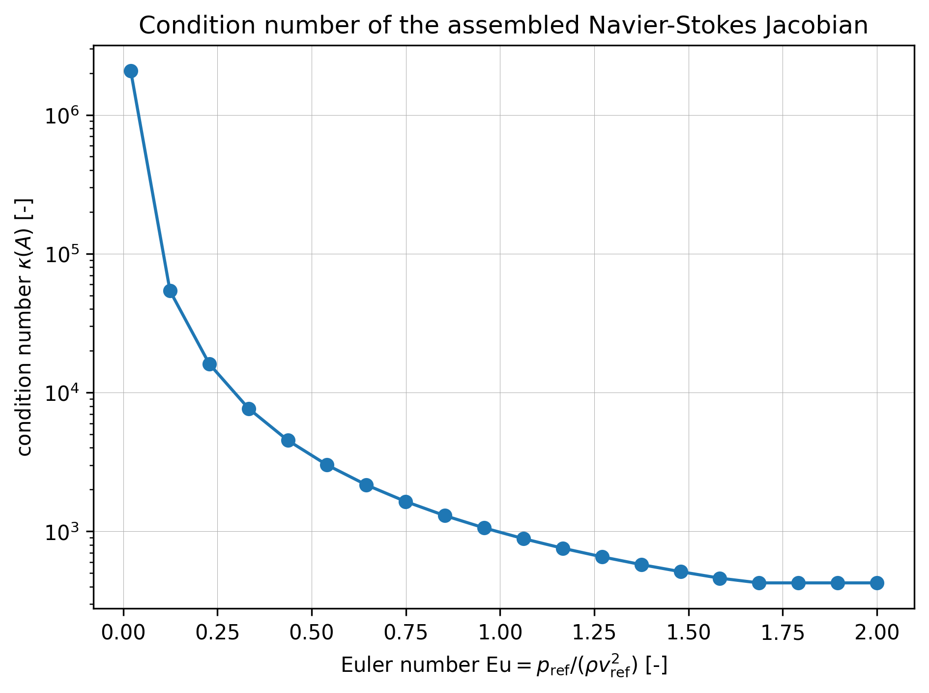
In the figure below, we observe that the condition number grows as the Euler number decreases. This is expected since is the coefficient of the pressure term in the normalized form, and the pressure term is responsible for the incompressibility constraint, and in turn the invertibility of the entire saddle-point Jacobian. In addition, for the condition number is at its lowest value and does not vary. This is because the pressure coefficient has a sufficiently large norm to ensure good conditioning, and what determines the condition number in this regime is the lowest singular value of the velocity-velocity block, see Section 4.1 of Habera & Zilian (2026) for more details.
Source
forms = ufl.extract_blocks(form_nondimensional)  # type: ignore[arg-type]
problem = dolfiny.snesproblem.SNESProblem(forms, [v, p], bcs=bcs, prefix="ns", nest=False)

with problem.x0.localForm() as x_local:
    x_local.set(0.0)


def assemble_numpy_matrix(problem: dolfiny.snesproblem.SNESProblem) -> np.ndarray:
    """Assemble the Jacobian A into a dense NumPy array for condition-number estimates."""
    problem._J_block(problem.snes, problem.x0, problem.J, problem.J)
    return np.asarray(dolfiny.la.petsc_to_scipy(problem.J).toarray())


p_ref_values = np.linspace(args.p_ref_min, args.p_ref_max, args.num_p_ref)
condition_numbers = np.empty_like(p_ref_values)
# Euler number Eu = p_ref / (rho v_ref^2) along the pressure-scale sweep.
euler_values = p_ref_values / (float(rho.value) * float(v_ref.value) ** 2)

for i, p_ref_value in enumerate(p_ref_values):
    p_ref.scale = float(p_ref_value)
    condition_numbers[i] = np.linalg.cond(assemble_numpy_matrix(problem))

if comm.rank == 0:
    plt.figure(dpi=300)
    plt.title("Condition number of the assembled Navier-Stokes Jacobian")
    plt.xlabel(r"Euler number $\mathrm{Eu} = p_\mathrm{ref} / (\rho v_\mathrm{ref}^2)$ [-]")
    plt.ylabel(r"condition number $\kappa(A)$ [-]")
    plt.grid(linewidth=0.25)
    plt.semilogy(euler_values, condition_numbers, "o-")
    plt.tight_layout()
    plt.savefig(args.plot_file)
Figure 1:Condition number of the Jacobian of the normalized mixed Navier-Stokes residual, assembled at the zero state with cavity boundary conditions, as a function of the Euler number.
- Habera, M., & Zilian, A. (2026). Automated dimensional analysis for PDEs. arXiv. 10.48550/ARXIV.2601.06535